baseballr has provided two functions to pull statlines for players over custom date ranges, daily_batter_bref and daily_pitcher_bref. Unfortunately, Baseball-Reference has made some underlying changes to the feature that produces the data for those functions and I am not sure they will be salvageable any time soon.
In the meantime, as of baseballr 0.8.2, there is another way to get at this data. You can use the statline_from_statcast function to generate statlines over custom data ranges.
Here’s how to do it.
First, load the following packages:
library(baseballr)
library(tidyverse)
library(bpettir) # personal package available on GitHub, used for plotting
Next, you can either use Statcast data that you’ve previously acquired or pull the data directly from BaseballSavant. Let’s do the later. Say we want to see how players’ wOBA trend over rolling 7-day periods over the first 28 days of the 2019 season.
First you need to generate 7-day chunks of dates for the scrape_statcast_savant function, since that is the donwload limit. Note that I am ignoring the first two games played in Japan last year for simplicity:
dates <- seq.Date(as.Date('2019-03-28'),
                  as.Date('2019-04-24'), by = =7)

date_grid <- tibble(start_date = dates,
                    end_date = dates+6)

# # A tibble: 4 x 2
# start_date end_date
# <date>     <date>
# 1 2019-03-28 2019-04-03
# 2 2019-04-04 2019-04-10
# 3 2019-04-11 2019-04-17
# 4 2019-04-18 2019-04-24
We’ll use these start and end dates to repeately query BaseballSavant for the data. Here we use the map2_df function from the purrr package to create the repeated operation:
savant_data <- purrr::map2_df(.x = date_grid$start_date,
                              .y = date_grid$end_date,
                              ~scrape_statcast_savant(start_date = .x,
                                                      end_date = .y,
                                                      player_type = 'batter')
You should get a dataframe with 108202 observations.
Let’s create some batter statlines. We need to generate a list of unique batters:
batters <- savant_data %>%
  distinct(batter) %>%
  pull()
And now we can again use purrr to repeatedly apply the statline_from_statcast function to each batter in our data set, with two small tweaks. We can create a custom function that filters the data not only for the different batters, but also for the date ranges (7-day incremenets). Note that we are setting the base argument to ‘at bats’.
custom_statline <- function(df,
                            player,
                            start_date,
                            end_date) {

  df <- df %>%
    filter(batter == player) %>%
    filter(game_date >= start_date & game_date <= end_date)

  stats <- statline_from_statcast_beta(df,
                                       base = 'at bats')

  stats <- stats %>%
    mutate(batter = player)

  return(stats)
}
This function will filter the bulk data by player and then by date range.
We’ll expand our date grid to accomodate each batter to make the mapping easier. We need to create a slightly different grid to map over since what we want are 7-day rolling averages:
dates <- seq.Date(as.Date('2019-03-28'),
                  as.Date('2019-04-24'), by = 1)

date_grid <- tibble(start_date = dates,
                    end_date = dates+6)

date_grid <- date_grid %>%
  filter(end_date <= '2019-04-24')

batter_date_grid <- expand_grid(date_grid,
                                batters)
We now have a grid of 12694 combinations to run. That’s where the beauty of purrr::map makes things easy. We create a safe version of the functions, which will capture errors and continue operating over the grid rather than stopping if it encounters an error. We also make sure to name each element in the returned list with the end_date used (this will come in handy later). This should take around 6 minutes to run. You can probably speed this up, but that’s beyond the scope of this post:
safe_statline <- safely(custom_statline)

custom_statlines <- purrr::map(.x = seq(1, nrow(batter_date_grid), 1),
                        ~safe_statline(df = savant_data,
                                       player = batter_date_grid$batters[.x],
                                       start_date = batter_date_grid$start_date[.x],
                                       end_date = batter_date_grid$end_date[.x])
)

custom_statlines <- custom_statlines %>%
  set_names(batter_date_grid$end_date)
Finally, we want to merge in the names of the batters. We can use the get_chadwick_lu function to grab this information. We find the ‘result’ objects in our list, bind those results together, include the name of the list element as a column (so we know which time frame each applies to), and then join the player name to each:
player_info <- get_chadwick_lu()

player_info_reduced <- player_info %>%
  select(name_first, name_last, key_mlbam) %>%
  mutate(full_name = paste0(name_last, ', ', name_first))

custom_statlines_joined <- custom_statlines %>%
  purrr::map('result') %>%
  bind_rows(.id = 'seven_day_rolling_avg') %>%
  mutate(batter = as.numeric(batter)) %>%
  left_join(player_info_reduced, by = c('batter' = 'key_mlbam'))
And here’s the data!
glimpse(custom_statlines_joined)

# Observations: 12,694
# Variables: 20
# $ seven_day_rolling_avg <chr> "2019-04-03", "2019-04-03", "2019-04-03", "2019-04-03", "2019-04-03", "2…
# $ year                  <chr> "2019", "2019", "2019", "2019", "2019", "2019", "2019", "2019", "2019", …
# $ BB                    <dbl> 1, 1, 2, 3, 4, 2, 3, 2, 4, 2, 2, 3, 1, 2, 3, 5, 0, 0, 6, 2, 2, 3, 1, 0, …
# $ HBP                   <dbl> 0, 0, 0, 0, 1, 0, 0, 0, 3, 1, 0, 0, 0, 0, 2, 0, 0, 0, 0, 1, 0, 1, 0, 0, …
# $ SO                    <dbl> 1, 3, 3, 3, 2, 9, 0, 5, 1, 4, 2, 4, 5, 7, 2, 3, 5, 2, 3, 3, 2, 3, 1, 4, …
# $ X1B                   <dbl> 0, 0, 2, 2, 1, 3, 1, 3, 2, 5, 3, 1, 5, 4, 5, 1, 3, 0, 4, 2, 4, 3, 4, 0, …
# $ X2B                   <dbl> 0, 0, 0, 1, 0, 2, 1, 1, 0, 2, 0, 1, 0, 1, 1, 1, 2, 0, 0, 0, 1, 0, 2, 1, …
# $ X3B                   <dbl> 0, 0, 1, 0, 0, 0, 0, 0, 0, 0, 0, 0, 0, 0, 0, 0, 3, 0, 0, 0, 0, 0, 0, 0, …
# $ HR                    <dbl> 0, 0, 0, 1, 0, 1, 1, 2, 1, 2, 3, 1, 2, 0, 2, 1, 1, 0, 1, 0, 0, 0, 0, 0, …
# $ Outs                  <dbl> 2, 6, 14, 14, 6, 14, 1, 11, 13, 10, 9, 10, 16, 22, 16, 11, 14, 3, 13, 13…
# $ total_pas             <dbl> 3, 7, 19, 21, 12, 22, 7, 19, 23, 22, 17, 16, 24, 29, 29, 19, 23, 3, 24, …
# $ ba                    <dbl> 0.000, 0.000, 0.176, 0.222, 0.143, 0.300, 0.750, 0.353, 0.188, 0.474, 0.…
# $ obp                   <dbl> 0.333, 0.143, 0.263, 0.333, 0.500, 0.364, 0.857, 0.421, 0.435, 0.545, 0.…
# $ slg                   <dbl> 0.000, 0.000, 0.294, 0.444, 0.143, 0.550, 1.750, 0.765, 0.375, 0.895, 1.…
# $ ops                   <dbl> 0.333, 0.143, 0.557, 0.777, 0.643, 0.914, 2.607, 1.186, 0.810, 1.440, 1.…
# $ woba                  <dbl> 0.230, 0.099, 0.245, 0.332, 0.362, 0.380, 0.871, 0.478, 0.374, 0.580, 0.…
# $ batter                <dbl> 669738, 622569, 570481, 475582, 543776, 665742, 592567, 656941, 460086, …
# $ name_first            <chr> "Jake", "Pablo", "Erik", "Ryan", "JB", "Juan", "Colin", "Kyle", "Alex", …
# $ name_last             <chr> "Noll", "Reyes", "Gonzalez", "Zimmerman", "Shuck", "Soto", "Moran", "Sch…
# $ full_name             <chr> "Noll, Jake", "Reyes, Pablo", "Gonzalez, Erik", "Zimmerman, Ryan", "Shuc…
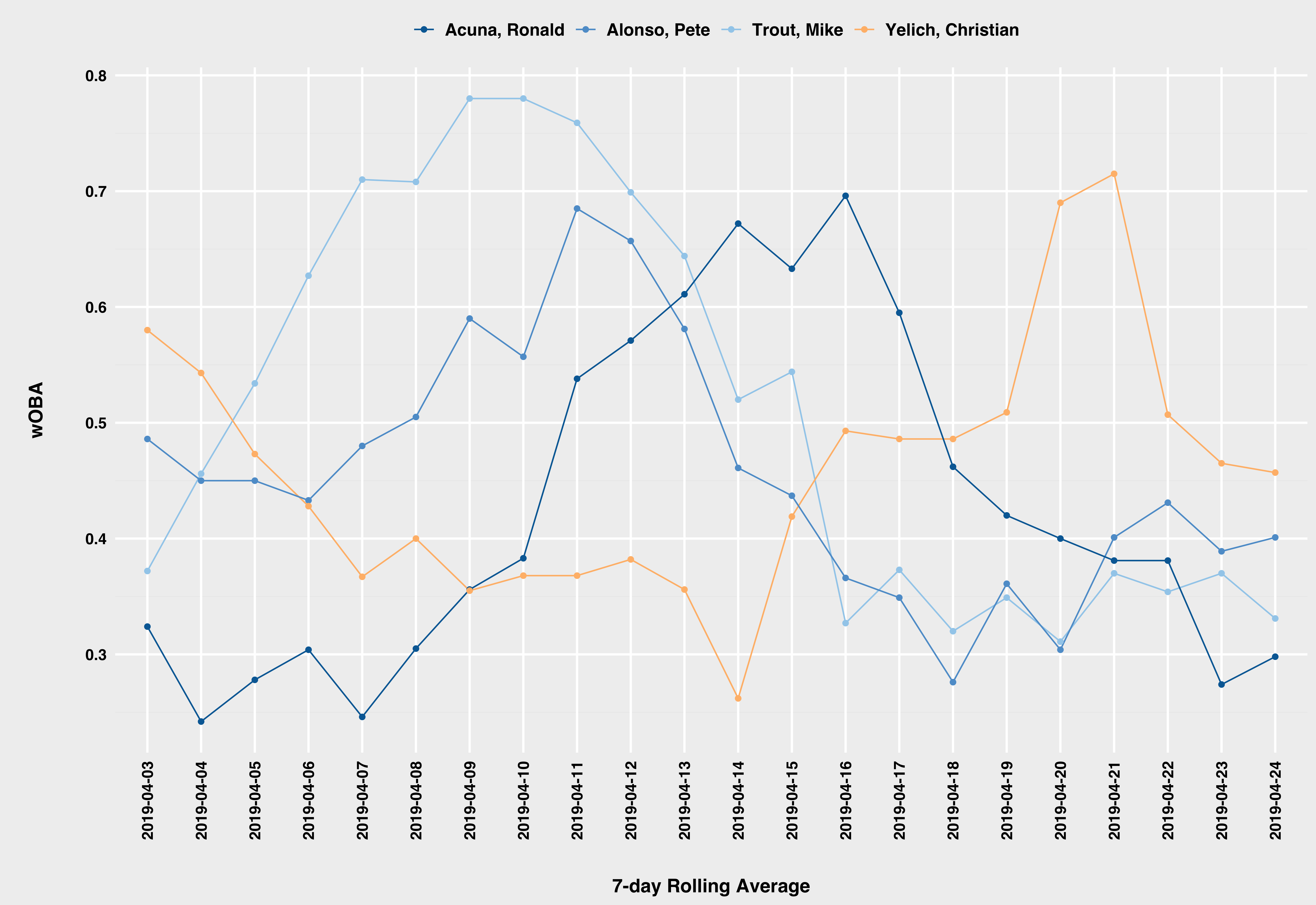
We can make some quick plots with it:
custom_statlines_joined %>%
  filter(batter %in% c(545361, 624413, 660670, 592885)) %>%
  ggplot(aes(seven_day_rolling_avg, woba, group = batter)) +
  geom_line(aes(color = full_name)) +
  geom_point(aes(color = full_name)) +
  scale_color_manual(values = tab_palette) +
  labs(x = '\n7-day Rolling Average',
       y = '\nwOBA\n') +
  theme_bp_grey() +
  theme(axis.text.x = element_text(angle = 90),
        legend.position = 'top',
        legend.title = element_blank())