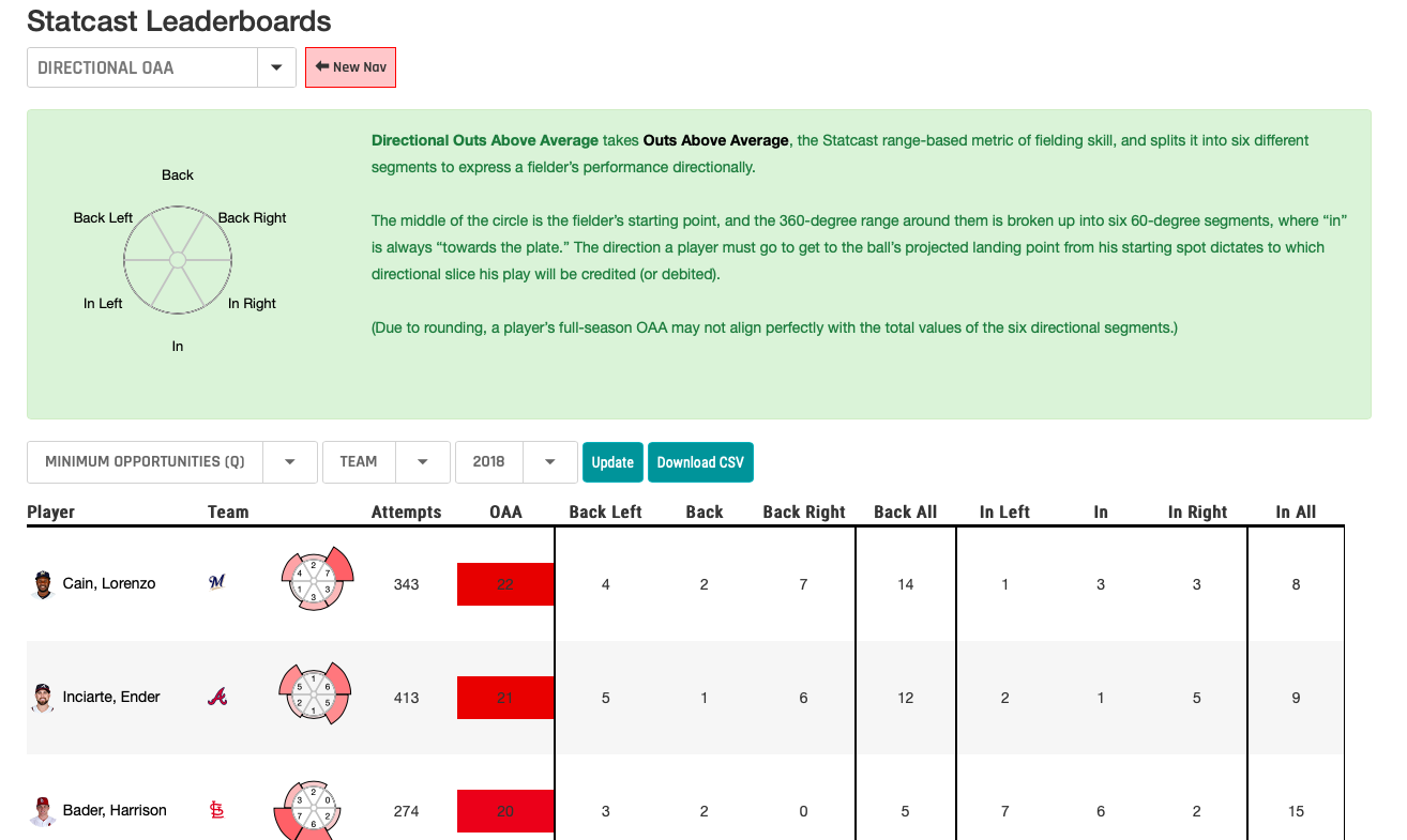
BaseballSavant recently made their series of leaderboards available through csv downloads. The baseballr package now includes a function that allows users to directly read these leaderboard csv’s into R.

The scrape_statcast_leaderboards() function can be used to access all of the leaderboards available as csv downloads. The function isn’t doing anything too sophisticated; it simply builds the appropriate url for the csv download based on a series of parameters and then reads the csv into R.
Users specificy which leaderboard they want to download using the leaderboard argument. The following are currently available:
exit_velocity_barrelsexpected_statisticspitch_arsenalouts_above_averagedirectional_oaacatch_probabilitypop_timesprint_speedrunning_splits_90_ft
Each leaderboard has different parameters that can be specific to alter the content of the downloads, but not all parameters work for every leaderboard. (I would check the leaderboard interface on BaseballSavant directly if you are not sure which ones to use.) Some of the leaderboards do not include a variable for the year selected, so the function will check if it exists and, if not, it will add a column based on your parameter setting.
Here is an example of the expected_statistics leaderboard for pitchers who faced at least 250 batters in 2018:
require(baseballr)
require(dplyr)
> payload <- scrape_savant_leaderboards(leaderboard = "expected_statistics",
+                            year = 2018,
+                            player_type = "pitcher",
+                            min_pa = 250)

> payload %>%
+   arrange(est_woba) %>%
+   select(year:last_name, pa, woba:est_woba_minus_woba_diff)
# A tibble: 274 x 6
    year last_name    pa  woba est_woba est_woba_minus_woba_diff
   <int> <chr>     <int> <dbl>    <dbl>                    <dbl>
 1  2018 Diaz        280 0.214    0.212                    0.002
 2  2018 Hader       306 0.219    0.229                   -0.01
 3  2018 Treinen     315 0.187    0.23                    -0.043
 4  2018 Ottavino    309 0.231    0.23                     0.001
 5  2018 Sale        617 0.237    0.232                    0.005
 6  2018 Verlander   833 0.26     0.236                    0.024
 7  2018 Betances    272 0.259    0.236                    0.023
 8  2018 Pressly     292 0.267    0.241                    0.026
 9  2018 deGrom      835 0.23     0.243                   -0.013
10  2018 Scherzer    866 0.252    0.246                    0.006
# ... with 264 more rows
You can also look at pop times for catchers with a minimum of 20 throws to second base:
> payload <- scrape_savant_leaderboards(leaderboard = "pop_time",
+                                       year = 2018,
+                                       min2b = 20)
> payload %>%
+   arrange(pop_2b_sb) %>%
+   select(year, catcher, exchange_2b_3b_sba, pop_2b_sba, pop_2b_cs, pop_2b_sb)
# A tibble: 36 x 6
    year catcher           exchange_2b_3b_sba pop_2b_sba pop_2b_cs pop_2b_sb
   <dbl> <chr>                          <dbl>      <dbl>     <dbl>     <dbl>
 1  2018 J.T. Realmuto                   0.69       1.9       1.88      1.9
 2  2018 Yan Gomes                       0.66       1.93      1.96      1.92
 3  2018 Austin Hedges                   0.7        1.94      1.92      1.95
 4  2018 Manny Pina                      0.67       1.94      1.93      1.95
 5  2018 Jorge Alfaro                    0.73       1.94      1.9       1.96
 6  2018 Willson Contreras               0.74       1.96      1.96      1.96
 7  2018 Salvador Perez                  0.68       1.98      1.98      1.96
 8  2018 Martin Maldonado                0.77       1.97      1.98      1.97
 9  2018 Luke Maile                      0.71       1.99      2.02      1.97
10  2018 Sandy Leon                      0.69       1.97      1.95      1.98
# ... with 26 more rows
New Phillie J.T. Realmuto had the fastest average pop time on stolen base attempts to second base at 1.90 seconds He was two one hundreths of a second faster when he caught a runner (1.88 vs. 1.90). As good as Jorge Alfaro is as a thrower, he trailed Realmuto by about four one hundreths on average, and Realmuto appeared to be more consistent with his pop times given the small difference between caught stealing and success steal times.
The one leaderboard not yet available through a csv download are the series of positional leaderboards. If and when they become available I will add them to the function.
If you run into any issues, please post a reproducible example here.