R Script for this Course
An R script that contains all the code below can be found here.
You can also download a pdf version of this course here.
What is R?
R is a programming language focused on manipulating and analyzing data.
R is also an open source language, meaning anyone can contribute to the R project, and develop and distribute code to run on the R platform
R has become one of the most popular languages used by statisticians and data scientists. As a result, there is a massive community that contributes to R.
In order to complete this crash course you will need R installed on your computer, as well as the RStudio IDE.
To download and install R, go to the CRAN homepage and following links to download and install.
To downloand and install RStudio, follow this link.
R Fundamentals
Working Directory
It’s always good to check and see where R will be saving your files–that includes data from your current session and any objects that you export from R (we’ll walk through that a little later)
To see what the current working directory is set to run getwd().
Note the use of forward slashes (“/”) in the path.
If you want to or need to change the default directory you can run setwd() and include the path you want. For example:
setwd("/whatever/path/you/want")
Assigning Objects
Objects can be assigned by using the <- operator.
foo <- "hello world!"
foo
## [1] "hello world!"
Object names should begin with a letter and can contain letters, numbers, underscores, or periods
When naming objects, remember that case matters:
myvar <- c(1,2,3)
Myvar
## Error in eval(expr, envir, enclos): object 'Myvar' not found
myvar
## [1] 1 2 3
Comments
Any text preceded by a # will be treated as a comment by R. That is, R will not try to execute it as code.
# This is a comment
# foo2 <- “hello world!”
foo2
## Error in eval(expr, envir, enclos): object 'foo2' not found
R throws an error because foo2 has not been assigned as an object in the environment, and that’s because we commented out the assignment.
Data Structures
Vectors
A vector in R is sequence of elements of the same type. They can be numeric:
x <- c(1,2,3,4,5)
x
## [1] 1 2 3 4 5
Or characters/strings:
firstNames <- c("Shinji", "Aska", "Rey", "Misato")
firstNames
## [1] "Shinji" "Aska" "Rey" "Misato"
Once a vector is saved as an object (i.e. variable), you can access different parts of the vector by referencing its indexed position.
For examnple, if we want the third name in the firstNames vector we run:
firstNames[3]
## [1] "Rey"
We can also explore the structure of a vector using the str() function:
str(firstNames)
## chr [1:4] "Shinji" "Aska" "Rey" "Misato"
Factors
Categorical variables in R are called “factors”. Factors have as many levels as their are unique categories.
# create a vector called 'gender'
gender <- c("f", "f", "f", "m", "m", "m", "m")
# transform 'gender' into a factor object
gender <- factor(gender)
# examine the structure of 'gender'
str(gender)
## Factor w/ 2 levels "f","m": 1 1 1 2 2 2 2
Lists
A list is a sequence of elements of different types. Below, we combine three vectors, each of a different type, into a single list:
myList <- list(x=x, firstNames=firstNames, gender=gender)
myList
## $x
## [1] 1 2 3 4 5
##
## $firstNames
## [1] "Shinji" "Aska"   "Rey"    "Misato"
##
## $gender
## [1] f f f m m m m
## Levels: f m
You can call specific elements within the list using the list index:
myList[[1]]
## [1] 1 2 3 4 5
Or execute functions on specific elements:
str(myList[[2]])
## chr [1:4] "Shinji" "Aska" "Rey" "Misato"
You can also reference individual elements from a list using $:
myList$x
## [1] 1 2 3 4 5
Or the name of the element with double branches
str(myList[['firstNames']])
## chr [1:4] "Shinji" "Aska" "Rey" "Misato"
Data frames
Data frames are two dimensional objects; think rows and columns.
Basically, data frames are tables of data. You can manually create data frames by combining two vectors with the data.frame function
franchise <- c("Mets", "Nationals", "Marlins", "Phillies", "Braves")
city <- c("New York", "Washington, DC", "Miami", "Philadelphia", "Atlanta")
teams <- data.frame(franchise, city)
teams
##   franchise           city
## 1      Mets       New York
## 2 Nationals Washington, DC
## 3   Marlins          Miami
## 4  Phillies   Philadelphia
## 5    Braves        Atlanta
Data frames are of class data.frame
The names of the columns (or variables) are stored as attributes of the data frame and can be called using names():
names(teams)
## [1] "franchise" "city"
Matrix, Matrices
A matrix is similar to a data frame except that all of its values are numeric.
Functions
Functions are pieces of codewritten to complete a specific, often repeated, task.
For example, if we wanted to find the mean of our x vector we could write the following code:
x
## [1] 1 2 3 4 5
(1+2+3+4+5)/5
## [1] 3
But this is inefficient, especially with a vector of any real length and complexity, so let’s write a function for it!
In R, functions consist of a function name and arguments. You feed the required arguments into the function and it returns a single value.
Let’s take the combine (or c) function that you’ve seen earlier, but I’ve failed to explain:
#combine the following elements into a vector: 1, 2, 3, 4, 5
x <- c(1, 2, 3, 4, 5)
x
## [1] 1 2 3 4 5
In the example above, c is the function name and everything in parenteses () are its arguments
Let’s go back to our mean example. R does have a base function built in for calculating means, but let’s build our own.
To do this, we will make use of some other base R functions:sum and length.
sum() takes whatever values are passed to it in its arguments and sums them.
length() returns the length (or count) of values passed to it in its arguments.
So here’s our version of a function for calculating the mean of a vector (and how you write a function, generally):
our.mean <- function(x){
  return(sum(x) / length(x))
}
So our function’s name is our.mean. It takes a vector or set of numbers as its arguments, sums those numbers and then divides that sum by the number of individual numbers returning the mean (average) of the set of numbers.
Let’s try it!
Here’s the mean of our x vector using R’s base mean() function:
x
## [1] 1 2 3 4 5
mean(x)
## [1] 3
And here’s the mean using the our.mean() function:
our.mean(x)
## [1] 3
We can even double check that these values are equivalent
mean(x) == our.mean(x)
## [1] TRUE
Let’s take another look at that function we wrote:
our.mean
## function(x){
##   return(sum(x) / length(x))
## }
The operations that should be applied are placed inside curly brackets {}.
Here we also used the return function to tell the function what should be returned to the environment after running.
There are other ways to make sure your result is returned to the environment.
Here are some additional examples:
our.mean <- function(x){
  foo <- sum(x) / length(x)
  print(foo)
}
or
our.mean <- function(x){
  foo <- sum(x) / length(x)
  foo
}
Both return 3 when applied to vector x
Functions can be very simple, like the our.mean function, or complex. You can layer in numerous functions and temporary objects.
For example, let’s say we wanted to summarize a vector in terms of it’s mean, median, and standard deviation:
our.summary <- function(x) {
  mean <- mean(x)
  median <- median(x)
  standard_deviation <- sd(x)
  foo <- cbind(mean, median, standard_deviation)
  return(foo)
}

our.summary(x)
##      mean median standard_deviation
## [1,]    3      3           1.581139
The function takes a vector and returns the three summary statistics we specified in the function. Notice that the function relies on other, pre-existing functions and only returns the outputs of those functions. It does not save the objects assigned inside the function to the global environment.
Take a look in your Environment pane, or use the function below to see a list of objects currently in your Environment:
ls()
##  [1] "city"        "firstNames"  "foo"         "franchise"   "gender"
##  [6] "myList"      "myvar"       "our.mean"    "our.summary" "teams"
## [11] "x"
Packages
Packages are essentially collections of functions that can be installed and loaded when necessary.
Anyone can write and distrbute a package, and they greatly expand R’s capabilities, and since they are open source R’s functionality expands very quickly.
Packages also allow for easy distribution and documentation of useful functions in all areas (data manipulation, modeling, visualiztion, web scraping, etc.).
R Packages are most commonly distributed through CRAN or through other outlets, e.g. GitHub.
Let’s use the example of reshape2 package.
reshape2 contains very useful functions for transforming datasets, for example from wide to long format and vice-versa
To install the reshape2 package from CRAN, use the install.packages function:
install.packages("reshape2")
library(reshape2)
You can see which packages are loaded by using the search function:
search()
##  [1] ".GlobalEnv"        "package:reshape2"  "package:stats"
##  [4] "package:graphics"  "package:grDevices" "package:utils"
##  [7] "package:datasets"  "package:methods"   "Autoloads"
## [10] "package:base"
You can also load packages using require().
Let’s first unload reshape2:
detach("package:reshape2")
Then use require and check to see if it loaded:
require(reshape2)
## Loading required package: reshape2
search()
##  [1] ".GlobalEnv"        "package:reshape2"  "package:stats"
##  [4] "package:graphics"  "package:grDevices" "package:utils"
##  [7] "package:datasets"  "package:methods"   "Autoloads"
## [10] "package:base"
Here are some of the packages I find most useful, day to day, some of which we will explore:
dplyr: robust functions for manipulating and summarizing tabular datareshape2: functions for transforming datasetsggplot2: comprehensive data visualization functionsggthemes: add*on forggplot2, providing custom graphic themesrvest: flexible web-scraping functions
More on packages later, just remember they are awesome.
Getting data in and out of R
There are several ways to get your data in and out of R. Let’s start with getting data in.
Base R includes a series of read. functions that can be used
- For csv files
read.delim("file location", header = TRUE, sep = "\t",
           quote = "\"", dec = ".", fill = TRUE, comment.char = "", ...)
- For other delimited files
read.delim("file location", header = TRUE, sep = "\t",
           quote = "\"", dec = ".", fill = TRUE, comment.char = "", ...)
You can also read in data that is stored on a website using the url of the site as the file location:
This is a csv file stored in a GitHub repositories:
dat <- read.csv("https://raw.githubusercontent.com/BillPetti/R-Crash-Course/master/FanGraphs_Leaderboard_Cum_WAR.csv",
                header = TRUE, na.strings="NA")
str(dat) will show you the structure of the object
str(dat)
## 'data.frame':	13988 obs. of  13 variables:
##  $ Season  : int  2000 1999 2015 2000 1998 1999 2014 2002 2008 2009 ...
##  $ Name    : Factor w/ 7571 levels "A.J. Burnett",..: 1 1 2 3 3 3 4 5 6 6 ...
##  $ Team    : Factor w/ 119 levels "- - -","Alleghenys",..: 61 61 71 110 110 110 80 95 7 7 ...
##  $ G       : int  13 7 3 33 7 9 2 9 22 23 ...
##  $ PA      : int  30 17 2 96 13 24 5 12 87 57 ...
##  $ wOBA    : num  0.375 0.106 0 0.353 0.319 0.316 0 0.081 0.309 0.208 ...
##  $ wRCplus : int  122 -50 -100 103 85 79 -100 -83 88 19 ...
##  $ BsR     : num  0 0 0 0.2 0 0 0 0 0.2 -0.1 ...
##  $ Off     : num  0.9 -3.5 -0.5 0.6 -0.3 -0.7 -1.2 -2.7 -1.1 -5.9 ...
##  $ Def     : num  3.5 1.9 0.2 2 -0.7 0.4 0.1 1.2 0.5 -1.8 ...
##  $ WAR     : num  0.5 -0.1 0 0.6 -0.1 0.1 -0.1 -0.1 0.2 -0.6 ...
##  $ Age     : int  23 22 23 23 21 22 23 23 22 23 ...
##  $ playerid: int  512 512 11467 746 746 746 11270 1571 4087 4087 ...
This is a good place to point out that, by default, R will read in any string variables as factors unless you tell it not to. If you look at the Name variable you can see that R has transformed it into a factor. In most cases you may not want that.
You can avoid this behavior by using the stringsAsFactors command.
Let’s try again:
dat <- read.csv("https://raw.githubusercontent.com/BillPetti/R-Crash-Course/master/FanGraphs_Leaderboard_Cum_WAR.csv",
                header = TRUE, na.strings="NA",
                stringsAsFactors = FALSE)

str(dat)
## 'data.frame':	13988 obs. of  13 variables:
##  $ Season  : int  2000 1999 2015 2000 1998 1999 2014 2002 2008 2009 ...
##  $ Name    : chr  "A.J. Burnett" "A.J. Burnett" "A.J. Cole" "A.J. Pierzynski" ...
##  $ Team    : chr  "Marlins" "Marlins" "Nationals" "Twins" ...
##  $ G       : int  13 7 3 33 7 9 2 9 22 23 ...
##  $ PA      : int  30 17 2 96 13 24 5 12 87 57 ...
##  $ wOBA    : num  0.375 0.106 0 0.353 0.319 0.316 0 0.081 0.309 0.208 ...
##  $ wRCplus : int  122 -50 -100 103 85 79 -100 -83 88 19 ...
##  $ BsR     : num  0 0 0 0.2 0 0 0 0 0.2 -0.1 ...
##  $ Off     : num  0.9 -3.5 -0.5 0.6 -0.3 -0.7 -1.2 -2.7 -1.1 -5.9 ...
##  $ Def     : num  3.5 1.9 0.2 2 -0.7 0.4 0.1 1.2 0.5 -1.8 ...
##  $ WAR     : num  0.5 -0.1 0 0.6 -0.1 0.1 -0.1 -0.1 0.2 -0.6 ...
##  $ Age     : int  23 22 23 23 21 22 23 23 22 23 ...
##  $ playerid: int  512 512 11467 746 746 746 11270 1571 4087 4087 ...
head(dat) shows the first 6 records or rows of the object:
head(dat)
##   Season            Name      Team  G PA  wOBA wRCplus BsR  Off  Def  WAR
## 1   2000    A.J. Burnett   Marlins 13 30 0.375     122 0.0  0.9  3.5  0.5
## 2   1999    A.J. Burnett   Marlins  7 17 0.106     -50 0.0 -3.5  1.9 -0.1
## 3   2015       A.J. Cole Nationals  3  2 0.000    -100 0.0 -0.5  0.2  0.0
## 4   2000 A.J. Pierzynski     Twins 33 96 0.353     103 0.2  0.6  2.0  0.6
## 5   1998 A.J. Pierzynski     Twins  7 13 0.319      85 0.0 -0.3 -0.7 -0.1
## 6   1999 A.J. Pierzynski     Twins  9 24 0.316      79 0.0 -0.7  0.4  0.1
##   Age playerid
## 1  23      512
## 2  22      512
## 3  23    11467
## 4  23      746
## 5  21      746
## 6  22      746
It is also possible to import specific file types, like excel or spss
For excel files, you can use the xlsx package:
require(xlsx)
df <- read.xlsx("<-name and extension of your file>", sheetIndex = 1)
SPSS files can be loaded with the help of the foreign package:
require(foreign)
df <- read.spss("file", use.value.labels = TRUE, to.data.frame = TRUE)
For SPSS files, if you want the value labels to be imported set the use.value.labels argument to TRUE; for the actual values, choose FALSE.
To export data, you simply use the write. series of functions.
# export a data frame as a csv file to your current working directory
write.csv(dat, "baseball_data.csv", row.names = FALSE)
# check your working directory for the file
You can also export to a different directory if you need to:
#export a data frame as a csv file to a different directory
write.csv(dat, "C:/Users/bill_petti/Documents/SomeNewFolder/baseball_data.csv",
          row.names = FALSE)
You can also export any object; for example, our summary table can be exported as a csv file :
summary.ex <- our.summary(x)
summary.ex
## mean median standard_deviation
## [1,]    3      3           1.581139
write.csv(summary.ex, "summary.ex.csv", row.names = FALSE)
You can also clean up your work space by removing objects (datasets, functions, etc.) using the rm() function.
A good rule of thumb is to remove any vectors that you have merged into data frames. Let’s remove the two vectors we used to ceate the teams data frame:
rm(city, franchise)
ls()
##  [1] "dat"         "firstNames"  "foo"         "gender"      "myList"
##  [6] "myvar"       "our.mean"    "our.summary" "teams"       "x"
You’ll notice that you can remove multiple objects at once by separating each with a comma.
You can remove all objects in your current environment by using the ls() function. This is a good idea when starting a new analysis to ensure you don’t end up referencing objects with similar names from a previous analysis.
rm(list=ls())
Manipulating data
Let’s walk through some common ways to manipulate data in R. We can use some of the datasets included in the base version. To see what’s available, execute data()
data()
Let’s load the iris dataset and view the first 10 rows:
data(iris)
head(iris, 3)
##   Sepal.Length Sepal.Width Petal.Length Petal.Width Species
## 1          5.1         3.5          1.4         0.2  setosa
## 2          4.9         3.0          1.4         0.2  setosa
## 3          4.7         3.2          1.3         0.2  setosa
We can access individual variables in a dataset using the $ notation. For example, say you just wanted to view the Sepal.Length variable from the iris dataset. If you try to call it directory, it won’t work:
head(Sepal.Length, 3)
## Error in head(Sepal.Length, 3): object 'Sepal.Length' not found
That’s because Sepal.Length isn’t a separate object; it only lives inside of the object iris.
Now, here’s how to access it using the $ notation:
head(iris$Sepal.Length, 3)
## [1] 5.1 4.9 4.7
If you want to access more than one variabe at a time you can make your life easier by using the with function.
with(iris, head(Sepal.Length, 3))
## [1] 5.1 4.9 4.7
The first argument in with is the data frame you want to reference, then you can identify individual variables simply by their name.
Here’s an example using multiple variables from the iris dataset. Let’s say we wanted to see the ratio of sepal length to width:
with(iris, Sepal.Length / Sepal.Width)
##   [1] 1.457143 1.633333 1.468750 1.483871 1.388889 1.384615 1.352941
##   [8] 1.470588 1.517241 1.580645 1.459459 1.411765 1.600000 1.433333
##  [15] 1.450000 1.295455 1.384615 1.457143 1.500000 1.342105 1.588235
##  [22] 1.378378 1.277778 1.545455 1.411765 1.666667 1.470588 1.485714
##  [29] 1.529412 1.468750 1.548387 1.588235 1.268293 1.309524 1.580645
##  [36] 1.562500 1.571429 1.361111 1.466667 1.500000 1.428571 1.956522
##  [43] 1.375000 1.428571 1.342105 1.600000 1.342105 1.437500 1.432432
##  [50] 1.515152 2.187500 2.000000 2.225806 2.391304 2.321429 2.035714
##  [57] 1.909091 2.041667 2.275862 1.925926 2.500000 1.966667 2.727273
##  [64] 2.103448 1.931034 2.161290 1.866667 2.148148 2.818182 2.240000
##  [71] 1.843750 2.178571 2.520000 2.178571 2.206897 2.200000 2.428571
##  [78] 2.233333 2.068966 2.192308 2.291667 2.291667 2.148148 2.222222
##  [85] 1.800000 1.764706 2.161290 2.739130 1.866667 2.200000 2.115385
##  [92] 2.033333 2.230769 2.173913 2.074074 1.900000 1.965517 2.137931
##  [99] 2.040000 2.035714 1.909091 2.148148 2.366667 2.172414 2.166667
## [106] 2.533333 1.960000 2.517241 2.680000 2.000000 2.031250 2.370370
## [113] 2.266667 2.280000 2.071429 2.000000 2.166667 2.026316 2.961538
## [120] 2.727273 2.156250 2.000000 2.750000 2.333333 2.030303 2.250000
## [127] 2.214286 2.033333 2.285714 2.400000 2.642857 2.078947 2.285714
## [134] 2.250000 2.346154 2.566667 1.852941 2.064516 2.000000 2.225806
## [141] 2.161290 2.225806 2.148148 2.125000 2.030303 2.233333 2.520000
## [148] 2.166667 1.823529 1.966667
What if we want the length/width ration to be a variable we can access in our dataset? You can assign variables to datasets using the $ notation:
iris$sepal_length_width_ratio <- with(iris, Sepal.Length / Sepal.Width)
head(iris)
##   Sepal.Length Sepal.Width Petal.Length Petal.Width Species
## 1          5.1         3.5          1.4         0.2  setosa
## 2          4.9         3.0          1.4         0.2  setosa
## 3          4.7         3.2          1.3         0.2  setosa
## 4          4.6         3.1          1.5         0.2  setosa
## 5          5.0         3.6          1.4         0.2  setosa
## 6          5.4         3.9          1.7         0.4  setosa
##   sepal_length_width_ratio
## 1                 1.457143
## 2                 1.633333
## 3                 1.468750
## 4                 1.483871
## 5                 1.388889
## 6                 1.384615
If you need to, you can also round values with the round function:
iris$sepal_length_width_ratio <- round(iris$sepal_length_width_ratio, 2)
head(iris)
##   Sepal.Length Sepal.Width Petal.Length Petal.Width Species
## 1          5.1         3.5          1.4         0.2  setosa
## 2          4.9         3.0          1.4         0.2  setosa
## 3          4.7         3.2          1.3         0.2  setosa
## 4          4.6         3.1          1.5         0.2  setosa
## 5          5.0         3.6          1.4         0.2  setosa
## 6          5.4         3.9          1.7         0.4  setosa
##   sepal_length_width_ratio
## 1                     1.46
## 2                     1.63
## 3                     1.47
## 4                     1.48
## 5                     1.39
## 6                     1.38
You can also recode variable using the ifelse function.
Let’s code each case based on whether they are below, between, or above the 1st and 3rd quartile for sepal_length_width_ratio:
You can get a quick summary of any variable with summary:
summary(iris$sepal_length_width_ratio)
##    Min. 1st Qu.  Median    Mean 3rd Qu.    Max.
##   1.270   1.550   2.030   1.954   2.228   2.960
iris$ratio_q <- with(iris,
     ifelse(sepal_length_width_ratio <= 1.550, 1,
     ifelse(sepal_length_width_ratio > 1.550 & sepal_length_width_ratio < 2.228, 2,
     ifelse(sepal_length_width_ratio >= 2.228, 3, NA))))
head(iris[,c(6:7)], 10)
##    sepal_length_width_ratio ratio_q
## 1                      1.46       1
## 2                      1.63       2
## 3                      1.47       1
## 4                      1.48       1
## 5                      1.39       1
## 6                      1.38       1
## 7                      1.35       1
## 8                      1.47       1
## 9                      1.52       1
## 10                     1.58       2
Subsetting Data
There are many ways to subset data in R. Let’s start with the base functions.
There are three unique species in the iris dataset. We can see unique values for any variable using the unique function:
unique(iris$Species)
## [1] setosa     versicolor virginica
## Levels: setosa versicolor virginica
Let’s say we wanted to subset iris and just include cases where the species is virginica. We can use the subset function:
sub_virginica <- subset(iris, Species == "virginica")
head(sub_virginica)
##     Sepal.Length Sepal.Width Petal.Length Petal.Width   Species
## 101          6.3         3.3          6.0         2.5 virginica
## 102          5.8         2.7          5.1         1.9 virginica
## 103          7.1         3.0          5.9         2.1 virginica
## 104          6.3         2.9          5.6         1.8 virginica
## 105          6.5         3.0          5.8         2.2 virginica
## 106          7.6         3.0          6.6         2.1 virginica
##     sepal_length_width_ratio ratio_q
## 101                     1.91       2
## 102                     2.15       2
## 103                     2.37       3
## 104                     2.17       2
## 105                     2.17       2
## 106                     2.53       3
unique(sub_virginica$Species)
## [1] virginica
## Levels: setosa versicolor virginica
Notice that in R the logical comparison for equals is ==.
We could also simply exclude all cases where Species == “virginica”.
ex_virginica <- subset(iris, Species != "virginica")
unique(ex_virginica$Species)
## [1] setosa     versicolor
## Levels: setosa versicolor virginica
We may also want to include more than one condition for the subset.
Let’s subset only those cases where Species == “virginica” and the legnth/width ratio is greater than 2:
sub_virginica2 <- subset(iris, Species != "virginica" & sepal_length_width_ratio >= 2)
head(sub_virginica2)
##    Sepal.Length Sepal.Width Petal.Length Petal.Width    Species
## 51          7.0         3.2          4.7         1.4 versicolor
## 52          6.4         3.2          4.5         1.5 versicolor
## 53          6.9         3.1          4.9         1.5 versicolor
## 54          5.5         2.3          4.0         1.3 versicolor
## 55          6.5         2.8          4.6         1.5 versicolor
## 56          5.7         2.8          4.5         1.3 versicolor
##    sepal_length_width_ratio ratio_q
## 51                     2.19       2
## 52                     2.00       2
## 53                     2.23       3
## 54                     2.39       3
## 55                     2.32       3
## 56                     2.04       2
You can also select specific variables using the index approach:
head(iris[,c(1,3)])
##   Sepal.Length Petal.Length
## 1          5.1          1.4
## 2          4.9          1.4
## 3          4.7          1.3
## 4          4.6          1.5
## 5          5.0          1.4
## 6          5.4          1.7
This returns just the first and third variables in the iris dataset.
You can also select specific cases using the same approach:
iris[c(1:6),]
##   Sepal.Length Sepal.Width Petal.Length Petal.Width Species
## 1          5.1         3.5          1.4         0.2  setosa
## 2          4.9         3.0          1.4         0.2  setosa
## 3          4.7         3.2          1.3         0.2  setosa
## 4          4.6         3.1          1.5         0.2  setosa
## 5          5.0         3.6          1.4         0.2  setosa
## 6          5.4         3.9          1.7         0.4  setosa
##   sepal_length_width_ratio ratio_q
## 1                     1.46       1
## 2                     1.63       2
## 3                     1.47       1
## 4                     1.48       1
## 5                     1.39       1
## 6                     1.38       1
This will return all variables in the dataset, but only rows one through six.
The dplyr package
While you can get very far with the base functions in R, I find the dplyr package to be a go-to tool for data manipulation.
dplyr was developed and is maintained by Hadley Wickham, who is currently the Chief Scientist at RStudio and has produced a number of the most prolific and useful R packages.
Much of the material that follows is borrowed from the in-depth vignette found here:
Let’s install and load it. This syntax below simply says that if R can’t load dplyr then install it first:
if (!require(dplyr)) {
install.packages(dplyr)
}
## Loading required package: dplyr
##
## Attaching package: 'dplyr'
## The following objects are masked from 'package:stats':
##
##     filter, lag
## The following objects are masked from 'package:base':
##
##     intersect, setdiff, setequal, union
To demonstratae the functionality of the dplyr package I’ve created a trimmed down version of the Lahman database, which is a publically available dataset of various baseball statistics.
To make life easier, there are two files (or tables) to import: lahman_reduced_batting and lahman_player:
batting <- read.csv("https://raw.githubusercontent.com/BillPetti/R-Crash-Course/master/batting_1950.csv",
                    header = TRUE,
                    stringsAsFactors = FALSE)

player <- read.csv("https://raw.githubusercontent.com/BillPetti/R-Crash-Course/master/player.csv",
                   header = TRUE,
                   stringsAsFactors = FALSE)
We can start by doing some basic subsetting using dplyr. You will see in many ways it is quite similar to some of the base R functionality.
We can filter for cases where a player had at least 600 at bats in a season using the filter function:
AB_400 <- filter(batting, AB >= 400)
We could also reduce the number of variables by using the select function:
AB_400_reduced <- select(AB_400, playerID, yearID, G, AB, HR)
Dplyr also allows you to create new variables using the mutate function:
AB_400 <- mutate(AB_400, AB_per_HR = AB/HR)
head(AB_400$AB_per_HR)
## [1] 80.60000 160.75000 54.20000 280.00000 37.50000 20.25926
You can use the arrange function to sort a data frame by a specific variable:
AB_400 <- arrange(AB_400, desc(HR))
head(AB_400$HR)
## [1] 73 70 66 65 64 63
dplyr also makes merging and joining differen datasets extremely easy.
Looking at the batting table you’ll notice that their is a playerID variable, but not the player’s actual name. That information is in the player table. Let’s look at the variables from that table:
str(player)
## 'data.frame':	18589 obs. of  26 variables:
##  $ playerID    : chr  "aardsda01" "aaronha01" "aaronto01" "aasedo01" ...
##  $ birthYear   : int  1981 1934 1939 1954 1972 1985 1854 1877 1869 1866 ...
##  $ birthMonth  : int  12 2 8 9 8 12 11 4 11 10 ...
##  $ birthDay    : int  27 5 5 8 25 17 4 15 11 14 ...
##  $ birthCountry: chr  "USA" "USA" "USA" "USA" ...
##  $ birthState  : chr  "CO" "AL" "AL" "CA" ...
##  $ birthCity   : chr  "Denver" "Mobile" "Mobile" "Orange" ...
##  $ deathYear   : int  NA NA 1984 NA NA NA 1905 1957 1962 1926 ...
##  $ deathMonth  : int  NA NA 8 NA NA NA 5 1 6 4 ...
##  $ deathDay    : int  NA NA 16 NA NA NA 17 6 11 27 ...
##  $ deathCountry: chr  NA NA "USA" NA ...
##  $ deathState  : chr  NA NA "GA" NA ...
##  $ deathCity   : chr  NA NA "Atlanta" NA ...
##  $ nameFirst   : chr  "David" "Hank" "Tommie" "Don" ...
##  $ nameLast    : chr  "Aardsma" "Aaron" "Aaron" "Aase" ...
##  $ nameGiven   : chr  "David Allan" "Henry Louis" "Tommie Lee" "Donald William" ...
##  $ weight      : int  205 180 190 190 184 220 192 170 175 169 ...
##  $ height      : int  75 72 75 75 73 73 72 71 71 68 ...
##  $ bats        : chr  "R" "R" "R" "R" ...
##  $ throws      : chr  "R" "R" "R" "R" ...
##  $ debut       : chr  "4/6/2004" "4/13/1954" "4/10/1962" "7/26/1977" ...
##  $ finalGame   : chr  "9/28/2013" "10/3/1976" "9/26/1971" "10/3/1990" ...
##  $ retroID     : chr  "aardd001" "aaroh101" "aarot101" "aased001" ...
##  $ bbrefID     : chr  "aardsda01" "aaronha01" "aaronto01" "aasedo01" ...
##  $ deathDate   : chr  NA NA "1984-08-16" NA ...
##  $ birthDate   : chr  "1981-12-27" "1934-02-05" "1939-08-05" "1954-09-08" ...
This table contains tons of biographical data about every player in the Lahman database. We can join the AB_400 table with this table, which will include the first and last name of each player among other variables.
We can use a left_join, which keeps all the cases from the first table and only matches in data from the second where there are common cases. playerID will be our key variable, which is simply the variable we use to match cases across both tables:
AB_400_names <- left_join(AB_400, player, by = "playerID")
Now that the players’ names are in the same dataset, let’s create a variable with both their first and last names using the paste function:
AB_400_names$fullName <- with(AB_400_names,
     paste(nameFirst, nameLast))
head(AB_400_names$fullName)
## [1] "Barry Bonds"  "Mark McGwire" "Sammy Sosa"   "Mark McGwire"
## [5] "Sammy Sosa"   "Sammy Sosa"
With dplyr, you can perform all standard types of joins, as well as use multiple criteria for the joins.
The variables you use for the join also do not need to have the same name.
Let’s remove the object we just created, change the name of the matching variable in the player object, and rejoin:
rm(AB_400_names)
names(player)[names(player) == "playerID"] <- "ID_number"
str(player)
## 'data.frame':	18589 obs. of  26 variables:
##  $ ID_number   : chr  "aardsda01" "aaronha01" "aaronto01" "aasedo01" ...
##  $ birthYear   : int  1981 1934 1939 1954 1972 1985 1854 1877 1869 1866 ...
##  $ birthMonth  : int  12 2 8 9 8 12 11 4 11 10 ...
##  $ birthDay    : int  27 5 5 8 25 17 4 15 11 14 ...
##  $ birthCountry: chr  "USA" "USA" "USA" "USA" ...
##  $ birthState  : chr  "CO" "AL" "AL" "CA" ...
##  $ birthCity   : chr  "Denver" "Mobile" "Mobile" "Orange" ...
##  $ deathYear   : int  NA NA 1984 NA NA NA 1905 1957 1962 1926 ...
##  $ deathMonth  : int  NA NA 8 NA NA NA 5 1 6 4 ...
##  $ deathDay    : int  NA NA 16 NA NA NA 17 6 11 27 ...
##  $ deathCountry: chr  NA NA "USA" NA ...
##  $ deathState  : chr  NA NA "GA" NA ...
##  $ deathCity   : chr  NA NA "Atlanta" NA ...
##  $ nameFirst   : chr  "David" "Hank" "Tommie" "Don" ...
##  $ nameLast    : chr  "Aardsma" "Aaron" "Aaron" "Aase" ...
##  $ nameGiven   : chr  "David Allan" "Henry Louis" "Tommie Lee" "Donald William" ...
##  $ weight      : int  205 180 190 190 184 220 192 170 175 169 ...
##  $ height      : int  75 72 75 75 73 73 72 71 71 68 ...
##  $ bats        : chr  "R" "R" "R" "R" ...
##  $ throws      : chr  "R" "R" "R" "R" ...
##  $ debut       : chr  "4/6/2004" "4/13/1954" "4/10/1962" "7/26/1977" ...
##  $ finalGame   : chr  "9/28/2013" "10/3/1976" "9/26/1971" "10/3/1990" ...
##  $ retroID     : chr  "aardd001" "aaroh101" "aarot101" "aased001" ...
##  $ bbrefID     : chr  "aardsda01" "aaronha01" "aaronto01" "aasedo01" ...
##  $ deathDate   : chr  NA NA "1984-08-16" NA ...
##  $ birthDate   : chr  "1981-12-27" "1934-02-05" "1939-08-05" "1954-09-08" ...
AB_400_names <- left_join(AB_400, player, by = c("playerID" = "ID_number"))
AB_400_names$fullName <- with(AB_400_names, paste(nameFirst, nameLast))
head(AB_400_names$fullName)
## [1] "Barry Bonds"  "Mark McGwire" "Sammy Sosa"   "Mark McGwire"
## [5] "Sammy Sosa"   "Sammy Sosa"
This is nice, but we probably want the player name as the first column. There are a few ways to rearrange column order in R.
Here are a few examples.
Let’s move fullName to the first column using the index approach
AB_400_names_index <- AB_400_names[,c(49, 1:48)]
head(AB_400_names_index[,c(1:6)])
##       fullName  playerID yearID stint teamID lgID
## 1  Barry Bonds bondsba01   2001     1    SFN   NL
## 2 Mark McGwire mcgwima01   1998     1    SLN   NL
## 3   Sammy Sosa  sosasa01   1998     1    CHN   NL
## 4 Mark McGwire mcgwima01   1999     1    SLN   NL
## 5   Sammy Sosa  sosasa01   2001     1    CHN   NL
## 6   Sammy Sosa  sosasa01   1999     1    CHN   NL
rm(AB_400_names_index)
We can also use the select function from dplyr:
AB_400_names_index <- select(AB_400_names, fullName, everything())
head(AB_400_names_index[,c(1:6)])
##       fullName  playerID yearID stint teamID lgID
## 1  Barry Bonds bondsba01   2001     1    SFN   NL
## 2 Mark McGwire mcgwima01   1998     1    SLN   NL
## 3   Sammy Sosa  sosasa01   1998     1    CHN   NL
## 4 Mark McGwire mcgwima01   1999     1    SLN   NL
## 5   Sammy Sosa  sosasa01   2001     1    CHN   NL
## 6   Sammy Sosa  sosasa01   1999     1    CHN   NL
Notice the use of everything(). This allows you to order whatever columns you want by name and then have the rest of the columns remain in their current order.
rm(AB_400_names_index)
The magic of piping
So far we have focused on discrete lines of code. In many cases you need to combine many lines of code to achieve some objective. But this can be inefficient, introduces more opportunity for error, and can make the code less readable–as well as increasing the number of objects in your environment.
Entering the pipe function, or %>%.
%>% basically means then. Do whatever operation is on the left side of the %>%, then do whatever is one the right using the data from the left.
Here is a basic example. Creat an object that only contains players whose height was less than 5’10” (or 70 inches) and then select only fullName, yearID, and HR:
AB_400_names_reduced <- filter(AB_400_names, height < 70) %>%
  select(fullName, yearID, HR)

head(AB_400_names_reduced)
##         fullName yearID HR
## 1 Roy Campanella   1953 41
## 2    Matt Stairs   1999 38
## 3 Ivan Rodriguez   1999 35
## 4  Miguel Tejada   2002 34
## 5  Miguel Tejada   2004 34
## 6 Roy Campanella   1951 33
You can also expand on this as much as you want. Let’s also arrange the data by HR in ascending order:
AB_400_names_reduced <- filter(AB_400_names, height < 70) %>%
  select(fullName, yearID, HR) %>%
  arrange(HR)

head(AB_400_names_reduced)
##          fullName yearID HR
## 1    Spook Jacobs   1954  0
## 2 Sparky Anderson   1959  0
## 3   Sonny Jackson   1967  0
## 4      Matty Alou   1968  0
## 5 Cesar Gutierrez   1970  0
## 6  Enzo Hernandez   1971  0
Reshape Data
Sometimes you need to change the orientation of your dataset. Some datasets are long–few columns, many rows; some datasets are wide–many columns, few rows.
The reshape2 packge makes these kinds of transformations very easy.
Let’s use the built in airquality dataset in R:
head(airquality)
##   Ozone Solar.R Wind Temp Month Day
## 1    41     190  7.4   67     5   1
## 2    36     118  8.0   72     5   2
## 3    12     149 12.6   74     5   3
## 4    18     313 11.5   62     5   4
## 5    NA      NA 14.3   56     5   5
## 6    28      NA 14.9   66     5   6
str(airquality)
## 'data.frame':	153 obs. of  6 variables:
##  $ Ozone  : int  41 36 12 18 NA 28 23 19 8 NA ...
##  $ Solar.R: int  190 118 149 313 NA NA 299 99 19 194 ...
##  $ Wind   : num  7.4 8 12.6 11.5 14.3 14.9 8.6 13.8 20.1 8.6 ...
##  $ Temp   : int  67 72 74 62 56 66 65 59 61 69 ...
##  $ Month  : int  5 5 5 5 5 5 5 5 5 5 ...
##  $ Day    : int  1 2 3 4 5 6 7 8 9 10 ...
Let’s create a long dataset from airquality:
long <- melt(airquality)
## No id variables; using all as measure variables
str(long)
## 'data.frame':	918 obs. of  2 variables:
##  $ variable: Factor w/ 6 levels "Ozone","Solar.R",..: 1 1 1 1 1 1 1 1 1 1 ...
##  $ value   : num  41 36 12 18 NA 28 23 19 8 NA ...
head(long)
##   variable value
## 1    Ozone    41
## 2    Ozone    36
## 3    Ozone    12
## 4    Ozone    18
## 5    Ozone    NA
## 6    Ozone    28
summary(long)
##     variable       value
##  Ozone  :153   Min.   :  1.00
##  Solar.R:153   1st Qu.:  8.00
##  Wind   :153   Median : 19.50
##  Temp   :153   Mean   : 56.02
##  Month  :153   3rd Qu.: 78.00
##  Day    :153   Max.   :334.00
##                NA's   :44
We have melted the dataset, creating one column that includes each column from the original dataset, and another column that contains each value of the previous variables for each case.
We went from 153 cases with 6 variables to 918 cases with 2 variables.
We can also customize what variables to keep in the melted data. Let’s keep Month and Day:
long <- melt(airquality, id.vars = c("Month", "Day"))
str(long)
## 'data.frame':	612 obs. of  4 variables:
##  $ Month   : int  5 5 5 5 5 5 5 5 5 5 ...
##  $ Day     : int  1 2 3 4 5 6 7 8 9 10 ...
##  $ variable: Factor w/ 4 levels "Ozone","Solar.R",..: 1 1 1 1 1 1 1 1 1 1 ...
##  $ value   : num  41 36 12 18 NA 28 23 19 8 NA ...
head(long)
##   Month Day variable value
## 1     5   1    Ozone    41
## 2     5   2    Ozone    36
## 3     5   3    Ozone    12
## 4     5   4    Ozone    18
## 5     5   5    Ozone    NA
## 6     5   6    Ozone    28
Now the data is melted, but we have multiple rows for each Month and Day combination–one for each variable.
We can transform the long dataset back to wide using the dcast function:
wide <- dcast(long, Month + Day ~ variable, value.var = c("value"))
head(wide)
##   Month Day Ozone Solar.R Wind Temp
## 1     5   1    41     190  7.4   67
## 2     5   2    36     118  8.0   72
## 3     5   3    12     149 12.6   74
## 4     5   4    18     313 11.5   62
## 5     5   5    NA      NA 14.3   56
## 6     5   6    28      NA 14.9   66
head(airquality)
##   Ozone Solar.R Wind Temp Month Day
## 1    41     190  7.4   67     5   1
## 2    36     118  8.0   72     5   2
## 3    12     149 12.6   74     5   3
## 4    18     313 11.5   62     5   4
## 5    NA      NA 14.3   56     5   5
## 6    28      NA 14.9   66     5   6
When we compare the wide dataset to the original airquality dataset the only difference is the order of the variables.
We can also cast long datasets and apply aggregating functions to them. Let’s say we want to get the mean for each measure by month in the long dataset:
mean_by_month <- dcast(long, Month ~ variable, value.var = c("value"), fun.aggregate = mean, na.rm = TRUE)
mean_by_month
##   Month    Ozone  Solar.R      Wind     Temp
## 1     5 23.61538 181.2963 11.622581 65.54839
## 2     6 29.44444 190.1667 10.266667 79.10000
## 3     7 59.11538 216.4839  8.941935 83.90323
## 4     8 59.96154 171.8571  8.793548 83.96774
## 5     9 31.44828 167.4333 10.180000 76.90000
There are easier ways to quickly aggregate variables in a dataset than melting, casting, and re-melting though, which brings us to descriptive and summary statistics.
Basic descriptive and summary statistics
The most basic way to get a summary of the data in an object is through the summary function:
summary(airquality)
##      Ozone           Solar.R           Wind             Temp
##  Min.   :  1.00   Min.   :  7.0   Min.   : 1.700   Min.   :56.00
##  1st Qu.: 18.00   1st Qu.:115.8   1st Qu.: 7.400   1st Qu.:72.00
##  Median : 31.50   Median :205.0   Median : 9.700   Median :79.00
##  Mean   : 42.13   Mean   :185.9   Mean   : 9.958   Mean   :77.88
##  3rd Qu.: 63.25   3rd Qu.:258.8   3rd Qu.:11.500   3rd Qu.:85.00
##  Max.   :168.00   Max.   :334.0   Max.   :20.700   Max.   :97.00
##  NA's   :37       NA's   :7
##      Month            Day
##  Min.   :5.000   Min.   : 1.0
##  1st Qu.:6.000   1st Qu.: 8.0
##  Median :7.000   Median :16.0
##  Mean   :6.993   Mean   :15.8
##  3rd Qu.:8.000   3rd Qu.:23.0
##  Max.   :9.000   Max.   :31.0
##
This gives us the minimum and maximum values for each variable, the 1st and 3rd quartiles, mean, median, and the number of missing values.
But we can do better than this, obviously.
Let’s say we want to get other measures, like standard deviation, for each of the variables. We can use dplyr’s summarise_each function
summarise_each(airquality, funs(sd(., na.rm = TRUE)))
##      Ozone  Solar.R     Wind    Temp    Month     Day
## 1 32.98788 90.05842 3.523001 9.46527 1.416522 8.86452
The . represents where the table should go for a given function. So, as you pipe the data in to the next step in your code, the position of that data can be fixed by where you place the..
What if we want to get the standard deviation for each variable for each month? dplyr’s group_by function makes this very simple.
We can first remove the Day column using select, since we really don’t want the standard deviation for the day of the month.
select(airquality, -Day) %>%
  group_by(Month) %>%
  summarise_each(funs(sd(., na.rm = TRUE)))
## # A tibble: 5 × 5
##   Month    Ozone   Solar.R     Wind     Temp
##   <int>    <dbl>     <dbl>    <dbl>    <dbl>
## 1     5 22.22445 115.07550 3.531450 6.854870
## 2     6 18.20790  92.88298 3.769234 6.598589
## 3     7 31.63584  80.56834 3.035981 4.315513
## 4     8 39.68121  76.83494 3.225930 6.585256
## 5     9 24.14182  79.11828 3.461254 8.355671
Or, we can find the mean by month. You will see that the results are identical to what we saw after melting our data with the reshape2 package:
select(airquality, -Day) %>%
  group_by(Month) %>%
  summarise_each(funs(mean(., na.rm = TRUE)))
## # A tibble: 5 × 5
##   Month    Ozone  Solar.R      Wind     Temp
##   <int>    <dbl>    <dbl>     <dbl>    <dbl>
## 1     5 23.61538 181.2963 11.622581 65.54839
## 2     6 29.44444 190.1667 10.266667 79.10000
## 3     7 59.11538 216.4839  8.941935 83.90323
## 4     8 59.96154 171.8571  8.793548 83.96774
## 5     9 31.44828 167.4333 10.180000 76.90000
Cross tabulation is also pretty easy in R.
You can run a simple crosstabulation using the table function. Let’s cross Species by Petal.Width from the iris dataset:
with(iris, table(Species, Petal.Width))
##             Petal.Width
## Species      0.1 0.2 0.3 0.4 0.5 0.6  1 1.1 1.2 1.3 1.4 1.5 1.6 1.7 1.8
##   setosa       5  29   7   7   1   1  0   0   0   0   0   0   0   0   0
##   versicolor   0   0   0   0   0   0  7   3   5  13   7  10   3   1   1
##   virginica    0   0   0   0   0   0  0   0   0   0   1   2   1   1  11
##             Petal.Width
## Species      1.9  2 2.1 2.2 2.3 2.4 2.5
##   setosa       0  0   0   0   0   0   0
##   versicolor   0  0   0   0   0   0   0
##   virginica    5  6   6   3   8   3   3
We rarely want counts. We can get row or column frequencies by feeding the table result into the prop.table function.
If you don’t specific a margin value it will return the proportion of each cross for the entire dataset. For row frequencies, use margin = 1. For column frequencies, use margin = 2.
with(iris, table(Species, Petal.Width)) %>%
  prop.table() %>%
  round(., 2)
##             Petal.Width
## Species       0.1  0.2  0.3  0.4  0.5  0.6    1  1.1  1.2  1.3  1.4  1.5
##   setosa     0.03 0.19 0.05 0.05 0.01 0.01 0.00 0.00 0.00 0.00 0.00 0.00
##   versicolor 0.00 0.00 0.00 0.00 0.00 0.00 0.05 0.02 0.03 0.09 0.05 0.07
##   virginica  0.00 0.00 0.00 0.00 0.00 0.00 0.00 0.00 0.00 0.00 0.01 0.01
##             Petal.Width
## Species       1.6  1.7  1.8  1.9    2  2.1  2.2  2.3  2.4  2.5
##   setosa     0.00 0.00 0.00 0.00 0.00 0.00 0.00 0.00 0.00 0.00
##   versicolor 0.02 0.01 0.01 0.00 0.00 0.00 0.00 0.00 0.00 0.00
##   virginica  0.01 0.01 0.07 0.03 0.04 0.04 0.02 0.05 0.02 0.02
with(iris, table(Species, Petal.Width)) %>%
  prop.table(margin = 1) %>%
  round(., 2)
##             Petal.Width
## Species       0.1  0.2  0.3  0.4  0.5  0.6    1  1.1  1.2  1.3  1.4  1.5
##   setosa     0.10 0.58 0.14 0.14 0.02 0.02 0.00 0.00 0.00 0.00 0.00 0.00
##   versicolor 0.00 0.00 0.00 0.00 0.00 0.00 0.14 0.06 0.10 0.26 0.14 0.20
##   virginica  0.00 0.00 0.00 0.00 0.00 0.00 0.00 0.00 0.00 0.00 0.02 0.04
##             Petal.Width
## Species       1.6  1.7  1.8  1.9    2  2.1  2.2  2.3  2.4  2.5
##   setosa     0.00 0.00 0.00 0.00 0.00 0.00 0.00 0.00 0.00 0.00
##   versicolor 0.06 0.02 0.02 0.00 0.00 0.00 0.00 0.00 0.00 0.00
##   virginica  0.02 0.02 0.22 0.10 0.12 0.12 0.06 0.16 0.06 0.06
with(iris, table(Species, Petal.Width)) %>%
  prop.table(margin = 2) %>%
  round(., 2)
##             Petal.Width
## Species       0.1  0.2  0.3  0.4  0.5  0.6    1  1.1  1.2  1.3  1.4  1.5
##   setosa     1.00 1.00 1.00 1.00 1.00 1.00 0.00 0.00 0.00 0.00 0.00 0.00
##   versicolor 0.00 0.00 0.00 0.00 0.00 0.00 1.00 1.00 1.00 1.00 0.88 0.83
##   virginica  0.00 0.00 0.00 0.00 0.00 0.00 0.00 0.00 0.00 0.00 0.12 0.17
##             Petal.Width
## Species       1.6  1.7  1.8  1.9    2  2.1  2.2  2.3  2.4  2.5
##   setosa     0.00 0.00 0.00 0.00 0.00 0.00 0.00 0.00 0.00 0.00
##   versicolor 0.75 0.50 0.08 0.00 0.00 0.00 0.00 0.00 0.00 0.00
##   virginica  0.25 0.50 0.92 1.00 1.00 1.00 1.00 1.00 1.00 1.00
It is much easier to view and export crosstabs if you transform them using as.data.frame.matrix:
cross_column_ex <- with(iris, table(Species, Petal.Width)) %>%
  prop.table(margin = 2) %>%
  round(., 2) %>%
  as.data.frame.matrix()

write.csv(cross_column_ex, "cross_column.csv")
Basic statistics and modeling
Let’s use some sample survey data:
survey_data <- read.csv("https://raw.githubusercontent.com/BillPetti/R-Crash-Course/master/survey_sample_data.csv",
                        header = TRUE,
                        stringsAsFactors = FALSE)

str(survey_data)
## 'data.frame':	116 obs. of  19 variables:
##  $ resp: int  1 2 3 4 5 6 7 8 9 10 ...
##  $ Q1  : int  NA 4 4 4 4 4 4 4 3 2 ...
##  $ Q2  : int  4 4 4 3 2 4 4 4 4 4 ...
##  $ Q3  : int  4 4 4 4 3 5 4 4 4 5 ...
##  $ Q4  : int  2 4 2 3 3 5 3 3 4 5 ...
##  $ Q5  : int  4 4 4 3 2 4 4 4 4 4 ...
##  $ Q6  : int  3 4 4 4 4 4 3 4 4 4 ...
##  $ Q7  : int  3 5 4 4 3 5 4 4 4 4 ...
##  $ Q8  : int  4 5 4 4 2 4 4 4 4 2 ...
##  $ Q9  : int  4 5 4 3 4 5 4 4 4 4 ...
##  $ Q10 : int  4 5 3 3 4 5 4 3 3 4 ...
##  $ Q11 : int  4 5 3 4 4 5 4 3 4 5 ...
##  $ Q12 : int  4 5 3 3 3 5 4 3 4 5 ...
##  $ Q13 : int  2 5 4 NA 4 4 4 4 4 4 ...
##  $ Q14 : int  3 4 4 NA 3 4 4 4 4 5 ...
##  $ Q15 : int  2 5 4 NA 3 5 4 4 4 4 ...
##  $ Q16 : int  3 5 4 NA 3 4 4 4 4 4 ...
##  $ Q17 : int  2 5 4 NA 3 5 4 4 4 4 ...
##  $ Q18 : int  2 4 4 NA 3 4 4 4 4 4 ...
There are 116 respondents and 18 questions. The questions are on a 5-point Likert scale, from Strongly Disagree to Strongly Agree
Correlation
The base function cor can be used to find basic correlations between variables. You must specific how cor should handle missing values.
The use argument can take several meanings (see ?cor for more), but here we will use pairwise.
with(survey_data, cor(Q1, Q2, use = "pairwise.complete.obs"))
## [1] 0.3530547
We have 18 variables, so if we want to get a bird’s eye view of how the variables relate to each other we can create a correlation grid.
survey_data_correlations <- cor(survey_data, use = "pairwise.complete.obs")

survey_data_correlations
##             resp          Q1          Q2          Q3         Q4
## resp  1.00000000 -0.09574453 -0.09733647 -0.06927669 0.01795184
## Q1   -0.09574453  1.00000000  0.35305467  0.27953659 0.36221136
## Q2   -0.09733647  0.35305467  1.00000000  0.49294523 0.40183804
## Q3   -0.06927669  0.27953659  0.49294523  1.00000000 0.37346757
## Q4    0.01795184  0.36221136  0.40183804  0.37346757 1.00000000
## Q5   -0.07752839  0.50846209  0.68679399  0.48080170 0.50026715
## Q6   -0.10278028  0.50208986  0.43154085  0.30821207 0.53276408
## Q7   -0.08832711  0.38903930  0.40990115  0.42963346 0.49161124
## Q8   -0.16738552  0.55464228  0.49531524  0.29114575 0.48968584
## Q9   -0.04792468  0.24476313  0.37436979  0.24123260 0.37747731
## Q10  -0.04345704  0.29432257  0.35034226  0.29628574 0.24596518
## Q11  -0.09095514  0.40251704  0.49943984  0.58215362 0.48073189
## Q12  -0.10156412  0.43468247  0.49420490  0.34318982 0.48406513
## Q13  -0.10592351  0.27706723  0.43079785  0.30535647 0.31148109
## Q14  -0.03791991  0.45469984  0.54780552  0.42215991 0.50875202
## Q15  -0.11532400  0.45134415  0.48812145  0.39130098 0.43639175
## Q16  -0.03364900  0.24978777  0.39987277  0.33436690 0.29376051
## Q17  -0.16957063  0.50759671  0.45858814  0.32303033 0.45183619
## Q18  -0.06560827  0.53360753  0.58682384  0.41673379 0.47430199
##               Q5         Q6          Q7         Q8          Q9         Q10
## resp -0.07752839 -0.1027803 -0.08832711 -0.1673855 -0.04792468 -0.04345704
## Q1    0.50846209  0.5020899  0.38903930  0.5546423  0.24476313  0.29432257
## Q2    0.68679399  0.4315408  0.40990115  0.4953152  0.37436979  0.35034226
## Q3    0.48080170  0.3082121  0.42963346  0.2911457  0.24123260  0.29628574
## Q4    0.50026715  0.5327641  0.49161124  0.4896858  0.37747731  0.24596518
## Q5    1.00000000  0.6151182  0.39198432  0.6624960  0.37239510  0.28291910
## Q6    0.61511824  1.0000000  0.24834717  0.4594599  0.27136256  0.14947073
## Q7    0.39198432  0.2483472  1.00000000  0.4462642  0.36022430  0.27971519
## Q8    0.66249597  0.4594599  0.44626416  1.0000000  0.44720357  0.27328675
## Q9    0.37239510  0.2713626  0.36022430  0.4472036  1.00000000  0.35053588
## Q10   0.28291910  0.1494707  0.27971519  0.2732867  0.35053588  1.00000000
## Q11   0.51993760  0.3700152  0.46023070  0.4153304  0.34770778  0.49856876
## Q12   0.59267070  0.4260840  0.35593275  0.5801349  0.41948485  0.58012688
## Q13   0.46166738  0.4434746  0.16890253  0.4240773  0.56452679  0.27571723
## Q14   0.66105914  0.4503442  0.36154432  0.6031554  0.41041430  0.42245336
## Q15   0.59532481  0.5134326  0.34943444  0.5201491  0.46600263  0.48584327
## Q16   0.52009580  0.3468950  0.31036252  0.3847740  0.21757136  0.32395321
## Q17   0.56056300  0.6095168  0.39172399  0.6356982  0.54460462  0.43795159
## Q18   0.74346877  0.5561488  0.48942990  0.6283656  0.34770199  0.34963908
##              Q11        Q12        Q13         Q14        Q15        Q16
## resp -0.09095514 -0.1015641 -0.1059235 -0.03791991 -0.1153240 -0.0336490
## Q1    0.40251704  0.4346825  0.2770672  0.45469984  0.4513441  0.2497878
## Q2    0.49943984  0.4942049  0.4307978  0.54780552  0.4881214  0.3998728
## Q3    0.58215362  0.3431898  0.3053565  0.42215991  0.3913010  0.3343669
## Q4    0.48073189  0.4840651  0.3114811  0.50875202  0.4363918  0.2937605
## Q5    0.51993760  0.5926707  0.4616674  0.66105914  0.5953248  0.5200958
## Q6    0.37001517  0.4260840  0.4434746  0.45034421  0.5134326  0.3468950
## Q7    0.46023070  0.3559327  0.1689025  0.36154432  0.3494344  0.3103625
## Q8    0.41533043  0.5801349  0.4240773  0.60315541  0.5201491  0.3847740
## Q9    0.34770778  0.4194848  0.5645268  0.41041430  0.4660026  0.2175714
## Q10   0.49856876  0.5801269  0.2757172  0.42245336  0.4858433  0.3239532
## Q11   1.00000000  0.6071194  0.3669644  0.50990212  0.4715965  0.4954887
## Q12   0.60711941  1.0000000  0.3134537  0.63880203  0.5379101  0.4434703
## Q13   0.36696442  0.3134537  1.0000000  0.45666710  0.6387456  0.2578720
## Q14   0.50990212  0.6388020  0.4566671  1.00000000  0.6264466  0.5863867
## Q15   0.47159650  0.5379101  0.6387456  0.62644657  1.0000000  0.4271233
## Q16   0.49548875  0.4434703  0.2578720  0.58638668  0.4271233  1.0000000
## Q17   0.44136250  0.5627799  0.6819639  0.65112168  0.7606402  0.3944430
## Q18   0.58088418  0.5873540  0.5195240  0.71383053  0.6382698  0.5608581
##             Q17         Q18
## resp -0.1695706 -0.06560827
## Q1    0.5075967  0.53360753
## Q2    0.4585881  0.58682384
## Q3    0.3230303  0.41673379
## Q4    0.4518362  0.47430199
## Q5    0.5605630  0.74346877
## Q6    0.6095168  0.55614876
## Q7    0.3917240  0.48942990
## Q8    0.6356982  0.62836555
## Q9    0.5446046  0.34770199
## Q10   0.4379516  0.34963908
## Q11   0.4413625  0.58088418
## Q12   0.5627799  0.58735398
## Q13   0.6819639  0.51952397
## Q14   0.6511217  0.71383053
## Q15   0.7606402  0.63826976
## Q16   0.3944430  0.56085812
## Q17   1.0000000  0.69561874
## Q18   0.6956187  1.00000000
But we don’t really want to have the respondent column included, so we can exclude and re-run.
survey_data_correlations <- select(survey_data, -resp) %>%
  cor(use = "pairwise.complete.obs")

survey_data_correlations
##            Q1        Q2        Q3        Q4        Q5        Q6        Q7
## Q1  1.0000000 0.3530547 0.2795366 0.3622114 0.5084621 0.5020899 0.3890393
## Q2  0.3530547 1.0000000 0.4929452 0.4018380 0.6867940 0.4315408 0.4099012
## Q3  0.2795366 0.4929452 1.0000000 0.3734676 0.4808017 0.3082121 0.4296335
## Q4  0.3622114 0.4018380 0.3734676 1.0000000 0.5002671 0.5327641 0.4916112
## Q5  0.5084621 0.6867940 0.4808017 0.5002671 1.0000000 0.6151182 0.3919843
## Q6  0.5020899 0.4315408 0.3082121 0.5327641 0.6151182 1.0000000 0.2483472
## Q7  0.3890393 0.4099012 0.4296335 0.4916112 0.3919843 0.2483472 1.0000000
## Q8  0.5546423 0.4953152 0.2911457 0.4896858 0.6624960 0.4594599 0.4462642
## Q9  0.2447631 0.3743698 0.2412326 0.3774773 0.3723951 0.2713626 0.3602243
## Q10 0.2943226 0.3503423 0.2962857 0.2459652 0.2829191 0.1494707 0.2797152
## Q11 0.4025170 0.4994398 0.5821536 0.4807319 0.5199376 0.3700152 0.4602307
## Q12 0.4346825 0.4942049 0.3431898 0.4840651 0.5926707 0.4260840 0.3559327
## Q13 0.2770672 0.4307978 0.3053565 0.3114811 0.4616674 0.4434746 0.1689025
## Q14 0.4546998 0.5478055 0.4221599 0.5087520 0.6610591 0.4503442 0.3615443
## Q15 0.4513441 0.4881214 0.3913010 0.4363918 0.5953248 0.5134326 0.3494344
## Q16 0.2497878 0.3998728 0.3343669 0.2937605 0.5200958 0.3468950 0.3103625
## Q17 0.5075967 0.4585881 0.3230303 0.4518362 0.5605630 0.6095168 0.3917240
## Q18 0.5336075 0.5868238 0.4167338 0.4743020 0.7434688 0.5561488 0.4894299
##            Q8        Q9       Q10       Q11       Q12       Q13       Q14
## Q1  0.5546423 0.2447631 0.2943226 0.4025170 0.4346825 0.2770672 0.4546998
## Q2  0.4953152 0.3743698 0.3503423 0.4994398 0.4942049 0.4307978 0.5478055
## Q3  0.2911457 0.2412326 0.2962857 0.5821536 0.3431898 0.3053565 0.4221599
## Q4  0.4896858 0.3774773 0.2459652 0.4807319 0.4840651 0.3114811 0.5087520
## Q5  0.6624960 0.3723951 0.2829191 0.5199376 0.5926707 0.4616674 0.6610591
## Q6  0.4594599 0.2713626 0.1494707 0.3700152 0.4260840 0.4434746 0.4503442
## Q7  0.4462642 0.3602243 0.2797152 0.4602307 0.3559327 0.1689025 0.3615443
## Q8  1.0000000 0.4472036 0.2732867 0.4153304 0.5801349 0.4240773 0.6031554
## Q9  0.4472036 1.0000000 0.3505359 0.3477078 0.4194848 0.5645268 0.4104143
## Q10 0.2732867 0.3505359 1.0000000 0.4985688 0.5801269 0.2757172 0.4224534
## Q11 0.4153304 0.3477078 0.4985688 1.0000000 0.6071194 0.3669644 0.5099021
## Q12 0.5801349 0.4194848 0.5801269 0.6071194 1.0000000 0.3134537 0.6388020
## Q13 0.4240773 0.5645268 0.2757172 0.3669644 0.3134537 1.0000000 0.4566671
## Q14 0.6031554 0.4104143 0.4224534 0.5099021 0.6388020 0.4566671 1.0000000
## Q15 0.5201491 0.4660026 0.4858433 0.4715965 0.5379101 0.6387456 0.6264466
## Q16 0.3847740 0.2175714 0.3239532 0.4954887 0.4434703 0.2578720 0.5863867
## Q17 0.6356982 0.5446046 0.4379516 0.4413625 0.5627799 0.6819639 0.6511217
## Q18 0.6283656 0.3477020 0.3496391 0.5808842 0.5873540 0.5195240 0.7138305
##           Q15       Q16       Q17       Q18
## Q1  0.4513441 0.2497878 0.5075967 0.5336075
## Q2  0.4881214 0.3998728 0.4585881 0.5868238
## Q3  0.3913010 0.3343669 0.3230303 0.4167338
## Q4  0.4363918 0.2937605 0.4518362 0.4743020
## Q5  0.5953248 0.5200958 0.5605630 0.7434688
## Q6  0.5134326 0.3468950 0.6095168 0.5561488
## Q7  0.3494344 0.3103625 0.3917240 0.4894299
## Q8  0.5201491 0.3847740 0.6356982 0.6283656
## Q9  0.4660026 0.2175714 0.5446046 0.3477020
## Q10 0.4858433 0.3239532 0.4379516 0.3496391
## Q11 0.4715965 0.4954887 0.4413625 0.5808842
## Q12 0.5379101 0.4434703 0.5627799 0.5873540
## Q13 0.6387456 0.2578720 0.6819639 0.5195240
## Q14 0.6264466 0.5863867 0.6511217 0.7138305
## Q15 1.0000000 0.4271233 0.7606402 0.6382698
## Q16 0.4271233 1.0000000 0.3944430 0.5608581
## Q17 0.7606402 0.3944430 1.0000000 0.6956187
## Q18 0.6382698 0.5608581 0.6956187 1.0000000
To make it easier to read, we can round each correlation.
survey_data_correlations <- round(survey_data_correlations, 3)

survey_data_correlations
##        Q1    Q2    Q3    Q4    Q5    Q6    Q7    Q8    Q9   Q10   Q11
## Q1  1.000 0.353 0.280 0.362 0.508 0.502 0.389 0.555 0.245 0.294 0.403
## Q2  0.353 1.000 0.493 0.402 0.687 0.432 0.410 0.495 0.374 0.350 0.499
## Q3  0.280 0.493 1.000 0.373 0.481 0.308 0.430 0.291 0.241 0.296 0.582
## Q4  0.362 0.402 0.373 1.000 0.500 0.533 0.492 0.490 0.377 0.246 0.481
## Q5  0.508 0.687 0.481 0.500 1.000 0.615 0.392 0.662 0.372 0.283 0.520
## Q6  0.502 0.432 0.308 0.533 0.615 1.000 0.248 0.459 0.271 0.149 0.370
## Q7  0.389 0.410 0.430 0.492 0.392 0.248 1.000 0.446 0.360 0.280 0.460
## Q8  0.555 0.495 0.291 0.490 0.662 0.459 0.446 1.000 0.447 0.273 0.415
## Q9  0.245 0.374 0.241 0.377 0.372 0.271 0.360 0.447 1.000 0.351 0.348
## Q10 0.294 0.350 0.296 0.246 0.283 0.149 0.280 0.273 0.351 1.000 0.499
## Q11 0.403 0.499 0.582 0.481 0.520 0.370 0.460 0.415 0.348 0.499 1.000
## Q12 0.435 0.494 0.343 0.484 0.593 0.426 0.356 0.580 0.419 0.580 0.607
## Q13 0.277 0.431 0.305 0.311 0.462 0.443 0.169 0.424 0.565 0.276 0.367
## Q14 0.455 0.548 0.422 0.509 0.661 0.450 0.362 0.603 0.410 0.422 0.510
## Q15 0.451 0.488 0.391 0.436 0.595 0.513 0.349 0.520 0.466 0.486 0.472
## Q16 0.250 0.400 0.334 0.294 0.520 0.347 0.310 0.385 0.218 0.324 0.495
## Q17 0.508 0.459 0.323 0.452 0.561 0.610 0.392 0.636 0.545 0.438 0.441
## Q18 0.534 0.587 0.417 0.474 0.743 0.556 0.489 0.628 0.348 0.350 0.581
##       Q12   Q13   Q14   Q15   Q16   Q17   Q18
## Q1  0.435 0.277 0.455 0.451 0.250 0.508 0.534
## Q2  0.494 0.431 0.548 0.488 0.400 0.459 0.587
## Q3  0.343 0.305 0.422 0.391 0.334 0.323 0.417
## Q4  0.484 0.311 0.509 0.436 0.294 0.452 0.474
## Q5  0.593 0.462 0.661 0.595 0.520 0.561 0.743
## Q6  0.426 0.443 0.450 0.513 0.347 0.610 0.556
## Q7  0.356 0.169 0.362 0.349 0.310 0.392 0.489
## Q8  0.580 0.424 0.603 0.520 0.385 0.636 0.628
## Q9  0.419 0.565 0.410 0.466 0.218 0.545 0.348
## Q10 0.580 0.276 0.422 0.486 0.324 0.438 0.350
## Q11 0.607 0.367 0.510 0.472 0.495 0.441 0.581
## Q12 1.000 0.313 0.639 0.538 0.443 0.563 0.587
## Q13 0.313 1.000 0.457 0.639 0.258 0.682 0.520
## Q14 0.639 0.457 1.000 0.626 0.586 0.651 0.714
## Q15 0.538 0.639 0.626 1.000 0.427 0.761 0.638
## Q16 0.443 0.258 0.586 0.427 1.000 0.394 0.561
## Q17 0.563 0.682 0.651 0.761 0.394 1.000 0.696
## Q18 0.587 0.520 0.714 0.638 0.561 0.696 1.000
Let’s assume that we are very interested in the strength of the correlation between Q5 and Q2. Q18 also has a very strong correlation to Q2 (.587) and to Q5 (.743). We can run a partial correlation to better understand the strength and direction of the relationship between Q5 and Q2 after controlling for Q18.
Let’s install and load the ppcor package:
if(!require("ppcor")){
install.packages("ppcor")
library(ppcor)
}
## Loading required package: ppcor
## Loading required package: MASS
##
## Attaching package: 'MASS'
## The following object is masked from 'package:dplyr':
##
##     select
dplyr::select(survey_data, Q5, Q2, Q18) %>%
  filter(complete.cases(.)) %>%
  with(., pcor.test(Q2, Q5, Q18))
##    estimate         p.value statistic   n gp  Method
## 1 0.4557204 0.0000003934981  5.393988 114  1 pearson
So, after controlling for Q18 the correlation between Q2 and Q5 drops from .687 to .456. What if we controlled for all of the additional variables?
survey_data %>%
  filter(complete.cases(.)) %>%
  with(., pcor.test(Q2, Q5, .[,c(2, 4, 5, 7:19)]))
##    estimate     p.value statistic   n gp  Method
## 1 0.2991328 0.003070371  3.039368 112 16 pearson
ANOVA
R also has built in functionality for ANOVA.
Let’s randomly assign our respondents to 1 of 3 groups. set.seed allows you to replicate the same values when using sample or any other function that randomly generates numbers:
set.seed(42)
survey_data$group <- sample(1:3, 116, replace = TRUE)
with(survey_data, table(group))
## group
##  1  2  3
## 33 38 45
First, we check if there are differences between the groups and their response to Q2:
q2_anova <- aov(Q2 ~ as.factor(group), survey_data)
summary(q2_anova)
##                   Df Sum Sq Mean Sq F value Pr(>F)
## as.factor(group)   2   0.90  0.4502   0.559  0.573
## Residuals        113  90.99  0.8052
The p-value is quite high, so the groups are not different.
However, if they p-value was significant we could use the Tukey Honest Significance Difference method to see which pairs differef from each other:
TukeyHSD(q2_anova, conf.level = .95)
##   Tukey multiple comparisons of means
##     95% family-wise confidence level
##
## Fit: aov(formula = Q2 ~ as.factor(group), data = survey_data)
##
## $`as.factor(group)`
##            diff        lwr       upr     p adj
## 2-1 -0.19856459 -0.7056654 0.3085363 0.6225370
## 3-1 -0.02020202 -0.5086272 0.4682231 0.9946943
## 3-2  0.17836257 -0.2911583 0.6478835 0.6400294
Obvioulsy, none of the pairs will show as significant, but you can see what the output will look like for future analyses.
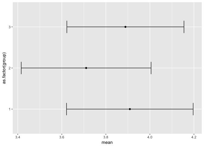
We could also have plotted the means and their confidence intervals and checked for overlaps (we are skipping ahead a bit to plotting, but oh well…)
group_means <- dplyr::select(survey_data, Q2, group) %>%
  filter(complete.cases(.)) %>%
  group_by(group) %>%
  summarise(mean = mean(Q2), sd = sd(Q2), Length = NROW(Q2), q2frac = qnorm(.975), Lower = mean - q2frac*sd/sqrt(Length), Upper = mean + q2frac*sd/sqrt(Length))

if(!require("ggplot2")){
install.packages("ggplot2")
require(ggplot2)
}
## Loading required package: ggplot2
## Warning: package 'ggplot2' was built under R version 3.3.2
ggplot(group_means, aes(x=mean, y=as.factor(group))) +
  geom_point() +
  geom_errorbarh(aes(xmin=Lower, xmax=Upper), height = .3)
Linear Regression
R has built-in functionality for running linear regressions witht the simple lm function.
Let’s download some new data and see what does a better job predicting the rate at which a pitcher will give up runs in the following season (ERA):
era <- read.csv("https://raw.githubusercontent.com/BillPetti/R-Crash-Course/master/pitchers150IP.csv",
                header = TRUE,
                stringsAsFactors = FALSE)
ERA_YR2 is our variable; it is a pitcher’s ERA in the following season.
First, let’s trim the data and take a look at a correlation grid between each variable and ERA in the following year:
era_yr2 <- era[,-c(1:2, 16)]

era_yr2_cor <- as.data.frame(cor(era_yr2))

data.frame(Metric = row.names(era_yr2_cor), ERA_YR2 = round(era_yr2_cor$ERA_YR2, 3)) %>%
  mutate(Rsquared = round(ERA_YR2^2,3)) %>%
  arrange(desc(Rsquared))
##             Metric ERA_YR2 Rsquared
## 1          ERA_YR2   1.000    1.000
## 2  K_minus_BB_perc  -0.413    0.171
## 3              FIP   0.413    0.171
## 4            SIERA   0.408    0.166
## 5           K_perc  -0.400    0.160
## 6             xFIP   0.397    0.158
## 7              ERA   0.357    0.127
## 8             WHIP   0.345    0.119
## 9              AVG   0.342    0.117
## 10            HR_9   0.250    0.062
## 11             LOB  -0.226    0.051
## 12         BB_perc   0.082    0.007
## 13           BABIP   0.075    0.006
## 14             E.F   0.014    0.000
Let’s run a linear model where ERA_YR2 is our outcome variable and we use all features in the data set:
era_lm <- lm(ERA_YR2 ~ ., data = era[,-c(1:2, 16)])

summary(era_lm)
##
## Call:
## lm(formula = ERA_YR2 ~ ., data = era[, -c(1:2, 16)])
##
## Residuals:
##      Min       1Q   Median       3Q      Max
## -1.56622 -0.48029 -0.06002  0.45769  2.36241
##
## Coefficients:
##                  Estimate Std. Error t value Pr(>|t|)
## (Intercept)       2.13289    3.60047   0.592   0.5539
## HR_9             -0.35338    1.05575  -0.335   0.7380
## K_perc          -67.92132   68.52679  -0.991   0.3222
## BB_perc          75.57925   68.05799   1.111   0.2674
## K_minus_BB_perc  66.49129   68.44015   0.972   0.3319
## AVG              15.10872   33.95992   0.445   0.6566
## WHIP             -2.55711    2.55804  -1.000   0.3181
## BABIP             0.33255   24.03978   0.014   0.9890
## LOB              -1.46977    2.21432  -0.664   0.5072
## ERA             -12.07430    7.01386  -1.721   0.0859 .
## FIP              12.62822    7.06305   1.788   0.0745 .
## E.F              12.08778    7.00692   1.725   0.0853 .
## xFIP              0.04712    0.41438   0.114   0.9095
## SIERA            -0.06316    0.48827  -0.129   0.8971
## ---
## Signif. codes:  0 '***' 0.001 '**' 0.01 '*' 0.05 '.' 0.1 ' ' 1
##
## Residual standard error: 0.7069 on 409 degrees of freedom
## Multiple R-squared:  0.2151,	Adjusted R-squared:  0.1901
## F-statistic:  8.62 on 13 and 409 DF,  p-value: 0.000000000000001423
You can also limit the predictor variables in the model by adding them to the model formula:
era_yr2_lm <- lm(ERA_YR2 ~ AVG + HR_9 + K_perc + K_minus_BB_perc, data = era_yr2)

summary(era_yr2_lm)
##
## Call:
## lm(formula = ERA_YR2 ~ AVG + HR_9 + K_perc + K_minus_BB_perc,
##     data = era_yr2)
##
## Residuals:
##     Min      1Q  Median      3Q     Max
## -1.6320 -0.4886 -0.0821  0.4702  2.4350
##
## Coefficients:
##                 Estimate Std. Error t value   Pr(>|t|)
## (Intercept)       3.1761     0.7072   4.491 0.00000918 ***
## AVG               3.8149     2.1472   1.777    0.07634 .
## HR_9              0.3697     0.1331   2.777    0.00574 **
## K_perc           -0.2520     2.1792  -0.116    0.90801
## K_minus_BB_perc  -5.3471     1.8632  -2.870    0.00432 **
## ---
## Signif. codes:  0 '***' 0.001 '**' 0.01 '*' 0.05 '.' 0.1 ' ' 1
##
## Residual standard error: 0.7057 on 418 degrees of freedom
## Multiple R-squared:  0.2007,	Adjusted R-squared:  0.1931
## F-statistic: 26.24 on 4 and 418 DF,  p-value: < 0.00000000000000022
You can call specific parts of the model output directly. For example, if you just wanted the coefficients of the model:
era_yr2_lm$coefficients
##     (Intercept)             AVG            HR_9          K_perc
##       3.1760902       3.8148715       0.3696733      -0.2519514
## K_minus_BB_perc
##      -5.3470963
The r and adjusted r squared needs to be called from the summary() of the model:
summary(era_yr2_lm)$adj.r.squared
## [1] 0.1930517
And you can apply the model to actual data using predict:
era_yr2_lm_predict <- predict(era_yr2_lm, era_yr2)

head(era_yr2_lm_predict)
##        1        2        3        4        5        6
## 3.292045 2.881584 2.940584 3.139357 2.500876 3.158717
If you aren’t applying to a new model you can just call the fit values from the model itself:
fit <- era_yr2_lm$fitted.values

head(fit)
##        1        2        3        4        5        6
## 3.292045 2.881584 2.940584 3.139357 2.500876 3.158717
We can calculate the accuracy of the model in terms of Mean Absolute Error (MAE) and Mean Absolute Percentage Error (MAPE):
compare <- data.frame(actual = era_yr2$ERA_YR2, predicted = fit)

compare$diff <- with(compare, predicted - actual)

MAE <- with(compare, mean(abs(diff)))

MAE
## [1] 0.5687383
MAPE <- with(compare, mean(abs(diff))/mean(actual))

MAPE
## [1] 0.1521268
How does this compare to just using ERA in Time1 to predict ERA in Time2?
with(era_yr2, mean(abs(ERA - ERA_YR2)))
## [1] 0.6950591
with(era_yr2, mean(abs(ERA - ERA_YR2))/mean(ERA_YR2))
## [1] 0.1859152
So our model increases the accuracy of just using ERA alone by about 18%:
round((0.1521268-.1859152)/.1859152,2)
## [1] -0.18
Plotting and data visualization
Base Plotting
Histograms
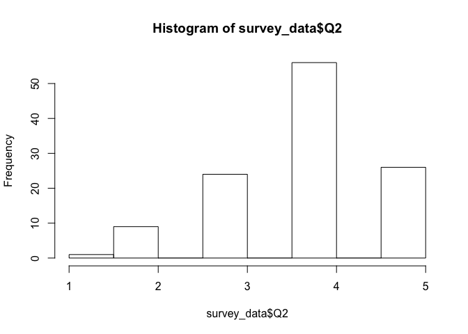
Creating histograms is extremely easy using the base plot functionality in R:
hist(survey_data$Q2)
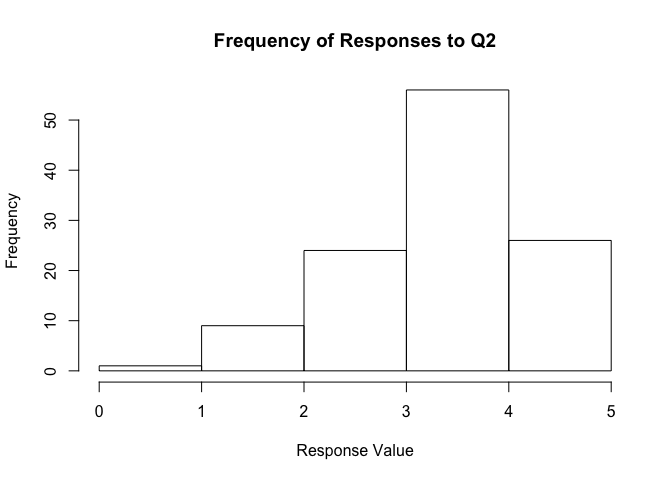
You can directly edit the breaks to be used:
hist(survey_data$Q2, main = "Frequency of Responses to Q2",
     xlab = "Response Value",
     breaks = c(0.0, 1.0, 2.0, 3.0, 4.0, 5.0))
You can also extract the values instead of the histogram:
hist(survey_data$Q2, breaks = c(0.0, 1.0, 2.0, 3.0, 4.0, 5.0),
     plot = FALSE)
## $breaks
## [1] 0 1 2 3 4 5
##
## $counts
## [1]  1  9 24 56 26
##
## $density
## [1] 0.00862069 0.07758621 0.20689655 0.48275862 0.22413793
##
## $mids
## [1] 0.5 1.5 2.5 3.5 4.5
##
## $xname
## [1] "survey_data$Q2"
##
## $equidist
## [1] TRUE
##
## attr(,"class")
## [1] "histogram"
Compare the $counts with a simple cross tab of Q2:
table(survey_data$Q2)
##
##  1  2  3  4  5
##  1  9 24 56 26
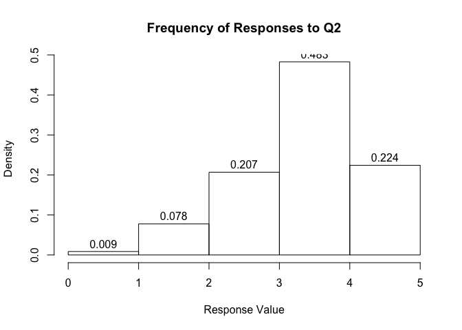
You can also show the density and not the counts for each bin:
hist(survey_data$Q2, main = "Frequency of Responses to Q2",
     xlab = "Response Value",
     breaks = c(0.0, 1.0, 2.0, 3.0, 4.0, 5.0),
     freq = FALSE,
     labels = TRUE)
You can further customize a hist through a variety of arguments. See ?hist for an accounting of the additional arguments.
Basic plots
Ccatter plots are also quite easy to generate:
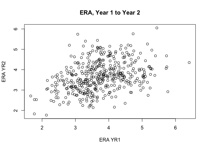
plot(ERA ~ ERA_YR2, data = era_yr2, main = "ERA, Year 1 to Year 2",
     xlab = "ERA YR1",
     ylab = "ERA YR2")
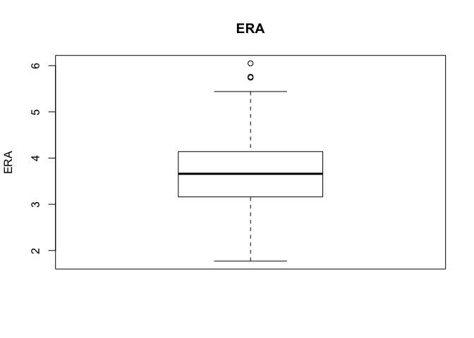
As are box plots:
boxplot(era_yr2$ERA, main = "ERA", ylab = "ERA")
ggplot2
R has pretty good base plotting options, but the beauty of plotting in R is the ggplot2 packge from Hadley Wickham (yep, there’s that name again).
With ggplot2, you are basically building the visual in layers. Plots can be saved as objects and then additional layers added on.
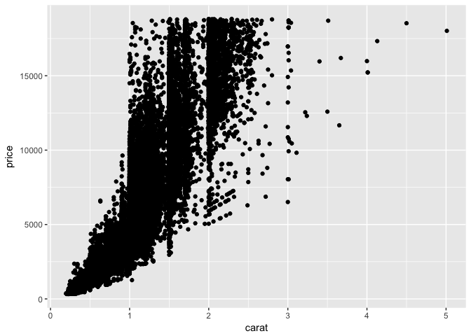
Let’s start with a basic scatterplot and use data from the diamonds data set:
ggplot(diamonds, aes(x = carat, y = price)) +
  geom_point()
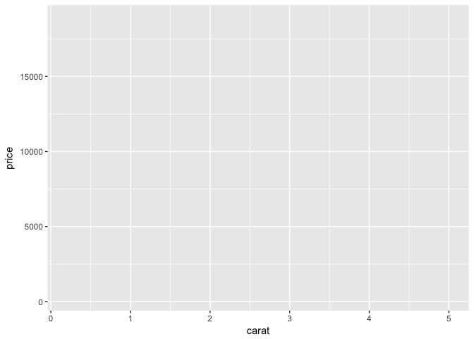
Let’s save the base of the plot as an object and then add additional layers one by one:
p <- ggplot(diamonds, aes(x = carat, y = price))
p
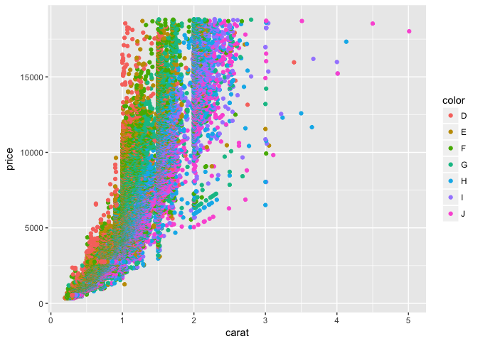
We can color code each point by the $color variable in the dataset:
p + geom_point(aes(color = color))
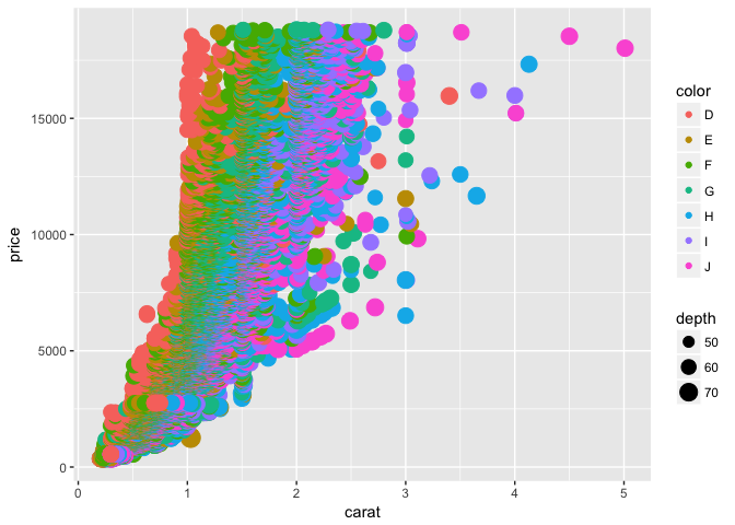
We could also adjust the size of each point by the depth variable
p + geom_point(aes(color = color, size = depth))
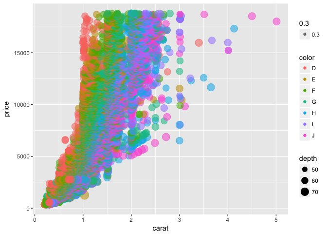
This is a bit hard to make out, so let’s add some transparency to each point using the alpha argument:
p + geom_point(aes(color = color, size = depth, alpha = .3))
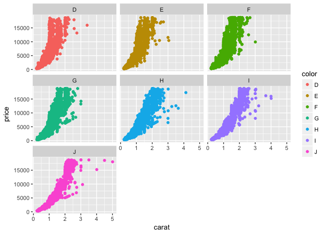
This still looks pretty messy, so let’s create separate plots to compare broken out by color. To do this, we can use the facet argument:
p + geom_point(aes(color = color)) +
  facet_wrap(~color)
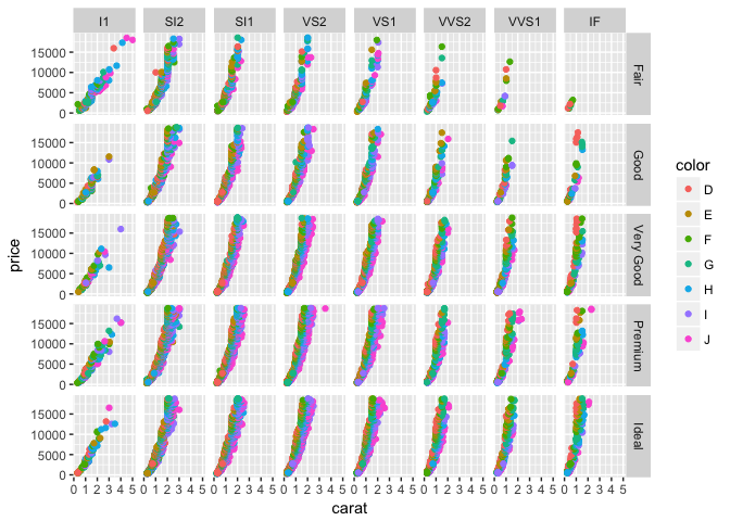
Facets can also work with two dimensions, and we can place the facets in a grid pattern:
p + geom_point(aes(color = color)) +
  facet_grid(cut ~ clarity)
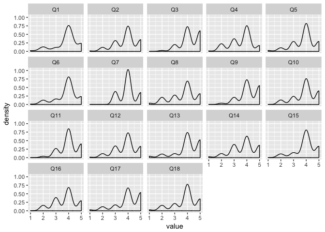
Faceting also makes it easy to view individual variables at once–for example, density plots for each survey question:
survey_data_melt <- melt(survey_data[,-c(1, 20)])
## No id variables; using all as measure variables
ggplot(survey_data_melt, aes(value)) + geom_density() + facet_wrap(~variable)
## Warning: Removed 16 rows containing non-finite values (stat_density).
ggplot2 also makes it easy to add a trend line to a scatter plot using stat_smooth:
p + geom_point() +
  stat_smooth()
## `geom_smooth()` using method = 'gam'
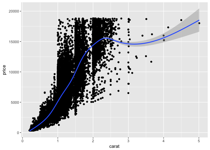
The grey shaded area is the confidence interval of the smoothed trend.
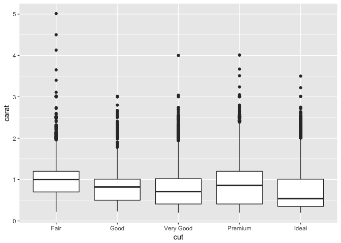
Here’s an example of boxplots in ggplot2:
ggplot(diamonds, aes(y = carat, x = cut)) +
  geom_boxplot()
Fleshing out a ggplot visual
There are many aspects of the plot that you can maipulate and customize in ggplot.
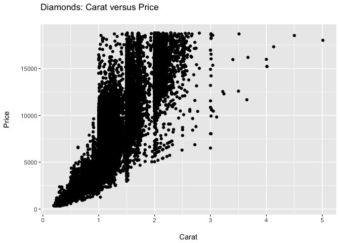
Going back to our saved p plot, we can add/edit a title, axis labels. The \n is a hard return that you can use to create more space between the labels and the plot:
pp <- p + geom_point() +
  ggtitle("Diamonds: Carat versus Price\n") +
  xlab("\nCarat") +
  ylab("Price\n")

pp
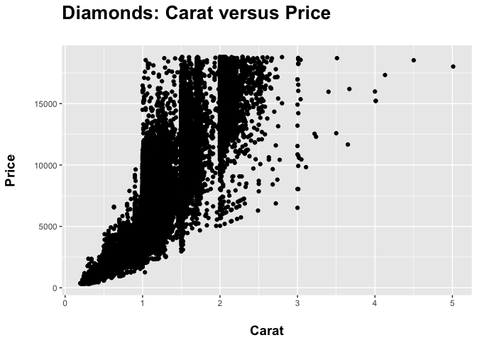
Formatting of text is accomplished by altering the theme of the plot.
Let’s bold the plot and axis titles and resize both, with the plot title being larger than the axis titles:
ppp <- pp + theme(axis.title = element_text(face = "bold", size = 14),
                  plot.title = element_text(face = "bold", size = 20))

ppp
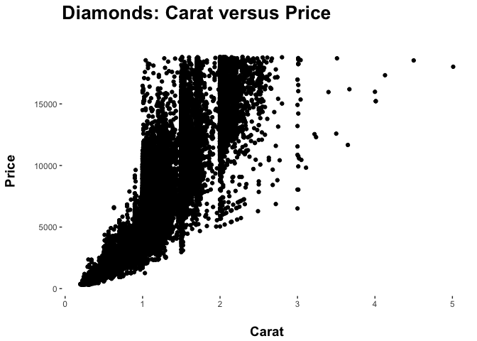
You can also remove elements of the plot via the theme() argument.
Let’s remove the shading of the plot usign element_blank():
pppp <- ppp + theme(panel.background = element_blank())

pppp
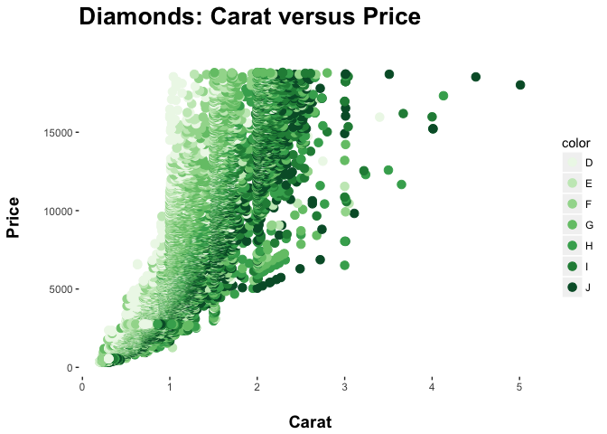
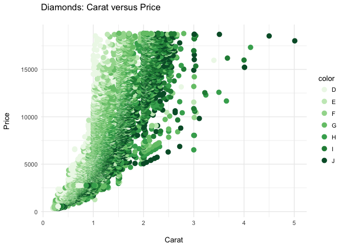
You can also use custom color palettes via a series of scale_ arguments.
Here we swap out the standard color palette for a palette of greens:
ppppp <- pppp + geom_point(aes(colour = color), size = 3) +
  scale_color_brewer(palette = "Greens")

ppppp
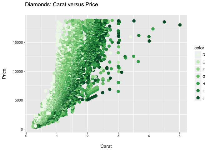
ggplot Themes
There are some built in variations of the basic theme in ggplot. You can easily swap them just by changing the theme() argument:
ppppp + theme_minimal()
ppppp + theme_bw()

ppppp + theme_grey()
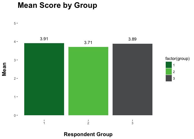
If you want, you can create your own palette of colors and use them in a plot as well:
g_palette <- c("#007934", "#61C250", "#595B5C")

ggplot(group_means, aes(factor(group), mean)) +
  geom_bar(stat = "identity", aes(fill = factor(group))) +
  geom_text(aes(label = round(mean,2), vjust = -1)) +
  scale_fill_manual(values = g_palette) +
  ggtitle("Mean Score by Group\n") +
  xlab("\nRespondent Group") +
  ylim(0,5) +
  ylab("Mean\n") +
  theme(axis.title = element_text(face = "bold", size = 14),
        plot.title = element_text(face = "bold", size = 20),
        panel.background = element_blank())
Correlation/R^2 Heatmap
Heatmaps are very useful, especially when looking at correlations across a series of variables in a data set.
Here’s some code to create one.
First, you need to calculate the correlation between all the variables in your data set, then melt the data:
survey_data_correlations_melt <- melt(cor(survey_data_correlations, use = "pairwise.complete.obs"))

survey_data_correlations_melt$value <-
  round(survey_data_correlations_melt$value, 2)
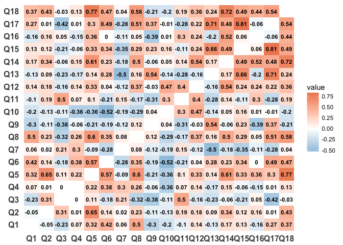
Then, we plot the data using geom_tile and scale_fill_gradient2 to scale the color of each tile based on its value:
ggplot(survey_data_correlations_melt, aes(Var1, Var2)) +
  geom_tile(aes(fill = value)) +
  geom_text(aes(label=value), size = 3, fontface = "bold") +
  scale_fill_gradient2(low = "#67a9cf", high = "#ef8a62") +
  theme_minimal() +
  theme(panel.grid.major = element_blank(),
        panel.grid.minor = element_blank(),
        panel.border = element_blank(),
        panel.background = element_blank(),
        axis.title = element_blank(),
        axis.text = element_text(size = 12, face = "bold"))
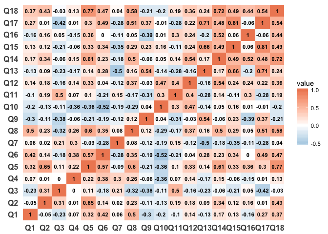
We should remove all values of 1 to make the heatmapping more intuititve and to display better
survey_data_correlations_melt <- survey_data_correlations_melt %>%
  filter(value < 1)

ggplot(survey_data_correlations_melt, aes(Var1, Var2)) +
  geom_tile(aes(fill = value)) +
  geom_text(aes(label=value), size = 3, fontface = "bold") +
  scale_fill_gradient2(low = "#67a9cf", high = "#ef8a62") +
  theme_minimal() +
  theme(panel.grid.major = element_blank(),
        panel.grid.minor = element_blank(),
        panel.border = element_blank(),
        panel.background = element_blank(),
        axis.title = element_blank(),
        axis.text = element_text(size = 12, face = "bold"))
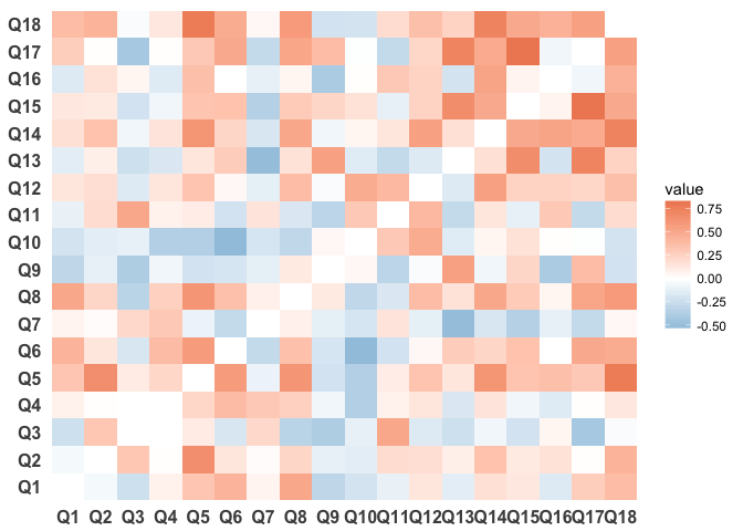
If the labels are distracting you can remove them:
ggplot(survey_data_correlations_melt, aes(Var1, Var2)) +
  geom_tile(aes(fill = value)) +
  scale_fill_gradient2(low = "#67a9cf", high = "#ef8a62") +
  theme_minimal() +
  theme(panel.grid.major = element_blank(),
        panel.grid.minor = element_blank(),
        panel.border = element_blank(),
        panel.background = element_blank(),
        axis.title = element_blank(),
        axis.text = element_text(size = 12, face = "bold"))
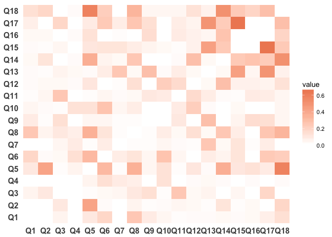
We could also plot the R^2 between questions:
survey_data_correlations_melt_r2 <- survey_data_correlations_melt %>%
  mutate(value = round(value^2, 2))

ggplot(survey_data_correlations_melt_r2, aes(Var1, Var2)) +
  geom_tile(aes(fill = value)) +
  scale_fill_gradient2(low = "#67a9cf", high = "#ef8a62") +
  theme_minimal() +
  theme(panel.grid.major = element_blank(),
        panel.grid.minor = element_blank(),
        panel.border = element_blank(),
        panel.background = element_blank(),
        axis.title = element_blank(),
        axis.text = element_text(size = 12, face = "bold"))
Additional Resources
As mentioned earlier, there are a ton of wonderful resources to help you get up to speed on R. Here are a few of my favorites.
Websites, etc.
-
List of the most useful R commands, Personality Project, http://www.personality-project/r/r.commands.html
-
Advanced R, Hadley Wickham, http://adv-r.had.co.nz/
-
dplyr vignettes, https://github.com/hadley/dplyr/blob/master/vignettes/introduction.Rmd
-
ggplot2 2.1.0 documentation, http://docs.ggplot2.org/current/
-
Interactive walkthrough of R for beginners: http://tryr.codeschool.com/
-
DataCamp course for R beginners: https://www.datacamp.com/courses/free-introduction-to-r
-
Swirl, an R package that walks you through lessons interactively from within R (may want to wait for the R crash course before wading into this if you have zero R experience): http://swirlstats.com/
-
Intro to R video playlist from Google: https://www.youtube.com/playlist?list=PLOU2XLYxmsIK9qQfztXeybpHvru-TrqAP
-
There is also a DataCamp course by Bob Muenchen, the author of R for SAS and SPSS Users. You can start it for free, but at some point you need to pay to advance through (not sure of the price): https://www.datacamp.com/courses/r-for-sas-spss-and-stata-users-r-tutorial
-
Twitter hashtag #rstats
Books
-
R for Everyone, Jared Lander, http://www.amazon.com/Everyone-Advanced-Analytics-Graphics-Addison-Wesley/dp/0321888030
-
R Cookbook, Paul Teetor, http://shop.oreilly.com/product/9780596809164.do
-
R in a Nutshell, Joseph Adler, http://shop.oreilly.com/product/0636920022008.do
-
An Introduction to Statistical Learning, Gareth James, et al, http://www-bcf.usc.edu/~gareth/ISL/ISLR%20First%20Printing.pdf
Acknowledgements
-
Bob Muenchen for beign kind enough to share the code that he uses when teaching a similar course. It was extremely helpful in setting up the content
-
Jared Lander’s great book, R for Everyone, was helpful to consult and was used for some of the
ggplot2and statistics examples -
Sean Anderson’s “An Introduction to reshape2” was used for the introduction to melting and casting data: http://seananderson.ca/2013/10/19/reshape.html